Open Journal of Statistics
Vol.1 No.1(2011), Article ID:4699,5 pages DOI:10.4236/ojs.2011.11003
Generalized Likelihood Ratio Tests for Varying-Coefficient Models with Censored Data
Department of Mathematics, Tongji University, Shanghai, 200092, P. R. China
E-mail: jrtrying@126.com
Received February 25, 2011; revised March 15, 2011; accepted March 23, 2011
Keywords: Varying Coefficient Model, Generalized Likelihood Ratio Test, Local Linear Method, Wilks Phenomenon, Censoring.
Abstract
In this paper, we extend the generalized likelihood ratio test to the varying-coefficient models with censored data. We investigate the asymptotic behavior of the proposed test and demonstrate that its limiting null distribution follows a  distribution, with the scale constant and the number of degree of freedom being independent of nuisance parameters or functions, which is called the wilks phenomenon. Both simulated and real data examples are given to illustrate the performance of the testing approach.
1. Introduction
Nonparametric regression model has become one of the main approaches in modern statistics due to its robustness and wide applications. In particular, it can be well estimated when the covariate is one dimension. However, as the dimension of the covariates, we face the phenomenon called "the curse of dimensionality". The varying coefficient model, which is the function approximation method for high dimension, is prosed (see Hastie and Tibshirani, 1993). Recently many statisticians (see Fan and Zhang 1999, 2000; Cai, 2007; Zhou and Ling, 2009; Wang and Xia, 2009; Chen and Tong, 2010) have investigated the varying coefficient model due to its simplifying structure, meaningful interpretation and wide application.
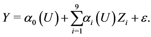
The varying-coefficient model has the following form:
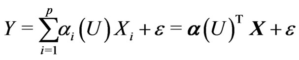 (1.1)
(1.1)
where ,
,  is unspecified smoothing function that needs to estimate,
  is random vector,
  is random variable, and its density function is
 ,
,  is random error, and
 ,
,
 .
.
However, in the real problems, for example, in the fields of reliable lifespan experiment, medicine track, survival analysis and so on,  can not be observed because it is censored. Let
  denotes the censoring random variable,
  and
and  are independent random variable under the condition that
  and
and  are given.
 ,
,  ,
, 
 , where
  denotes the sign function of a event, if
  is not censored, then
 , if
, if  is censored, then
 . We can only observe
 . Because responding variable is censored, we can not use the methods directly which we use on full data. So we should transform the data in an unbiased way to account for the censoring. An example of this kind is given in Buckley and James (1979). However, their transformation involves the unknow regression function leading to an iterative scheme. Motivated by the Buckley-James transformation, Koul, Susarla and Van Ryzin (1981) consider a transformation which only depends on the censoring distribution, but not on the regression function. Zheng (1987) proposed a class of transformations of this type. Once such a transformation is carried through, once can apply a variety of statistical techniques to analyze the transformed data as if they were uncensored. However, since such a transformation does not involve the distribution of the response variable, it increases the variability. Hence, some smoothing technique is necessary for modeling the transformed data. Some nonparametric regression techniques were applied in Dabrowska (1987) and Zheng (1988). In this paper, Class-K method is used to transform data.
In an effort to derive a generally applicable testing approach, Fan et al (2001) proposed the generalized likelihood ratio (GLR) statistic for nonparametric models. Their motivation was as follows. The maximum likelihood ratio test statistic in general may not exist in nonparametric and semiparametric settings. Even if it does, it is hard to find and may not be optimal in the simplest nonparametric regression setting. These drawbacks can be avoided when the maximum likelihood estimator is replaced by other reasonable nonparametric estimators, resulting in a class of statistics called the GLR statistic. The GLR test is intuitively appealing. Fan et al (2001) showed that for a variety of models and a number of nonparametric versus nonparametric and parametric versus nonparametric testing problems, the null distribution of the GLR test statistic follows an asymptotically distribution, independent of nuisance parameters. This property is called the Wilks phenomenon and facilitates the application of the GLR statistic. The critical value can be determined either by asymptotic distributions or by simulations. In this paper, we extend the generalized likelihood ratio test to the varyingcoefficient models with censored data.
The paper is organized as follows. Generalized likelihood ratio test is presented in section 2. In section 3, we provide two numerical results. Technical proofs are relegated to the Appendix.
2. Generalized Likelihood Ratio Tests
First, we replace the data point  with the transformed data point
  according to
 (2.1)
(2.1)
where  and
and  are the transformation functions. In the sequel of this paper we will refer to this transformation as the "ideal transformation", since it assumes that the transformation function
  and
and  are known. In practical situations however, those transformation functions typically have to be estimated. The estimations of
  and
and  can be expressed as (Fan and Gijbels, 1994)
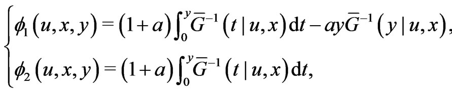 (2.2)
(2.2)
where  are respectively the conditional survival function of the random variable
  given
given  and
and . Remark that the Koul, Susarla and Van Ryzin (1981) transformation corresponds to
  and Leurgans (1987) transformation relates to
 . The tuning parameter
  in this New Class of transformations (2.2) creates the opportunity to improvement.
Starting from the transformed data
 , we now estimate the true regression functions
 . Fix a point
 approximate the unknown function:

This leads to the following weighted local least-squares problem: find  so as to minimize
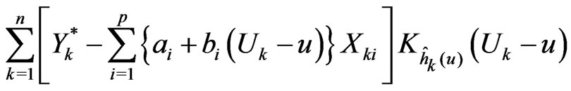 (2.3)
(2.3)
where  with K being a symmetric probability density function and we use the adaptive variable bandwidth of order k, and
 , here
  is the index of the design point
  closest to
 , the smoothing parameter
  can be obtained by cross-validation.
Let us work with the matrix notation. Denote ,
, ,
,  ,
,  denotes an
  matrix with
as its  th row, and
The solution to the problem (2.3) is given by
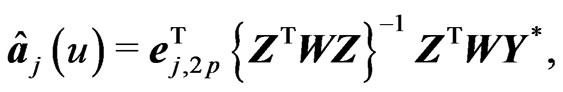
where  is the
  unit vector with 1 at the
  th position.
Consider the varying-coefficient model defined in (1.1). A nature question arises in practice is if these coefficient functions are really varying. This amounts to testing the following problem:
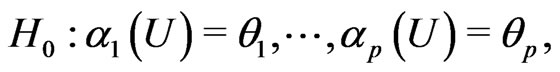
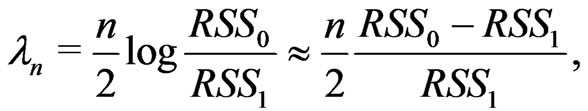
where  are unknown parameters. Following the same derivations as in Fan et al (2001), generalized likelihood ratio tests based on local linear fits are given by
where 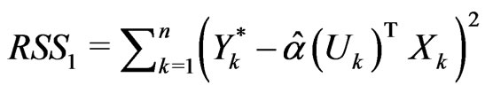 and
and 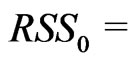
 with
with  is the least-square estimate under the null hypothesis.
We now describe our generalized Wilks type of theorem as follows:
Theorem 1 Suppose that conditions (C1)-(C5) given in the Appendix hold. Then, under , as
, as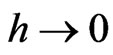 ,
,  ,
,
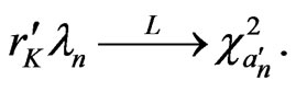
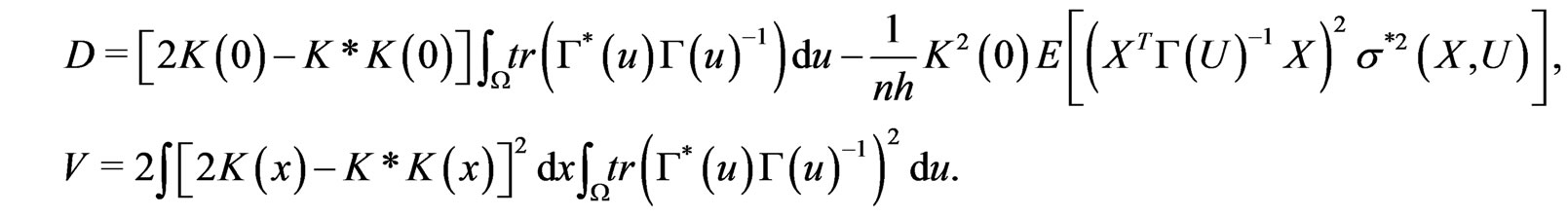
where  stands for convergence in distribution, and
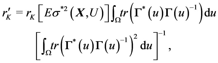
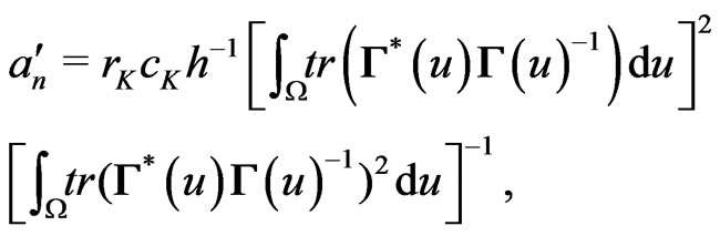
where ,
,
 ,
,
 ,
,
 ,
,
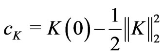
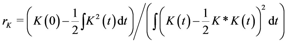 with
with  denote the convolution of K.
3. Numerical Studies
In this section, we first use Monte Carlo simulation studies to assess the finite sample performance of the test procedure proposed and then demonstrate the application of the method proposed by using a real data example. The programs are written in Matlab and are available upon request from the authors.
3.1. Simulation Example
Simulation data are generated from the varyingcoefficient partially linear model with censored data:
 (3.1)
(3.1)
where the covariate  is uniformly distributed on
 , the covariates
  are normally distributed with mean 0 and variance 1 and the distribution function of
  is
is , where
  or
or .
.  and
and  are simulated independently. The censoring variable
 . We vary
  to produce difference censoring rates(CR). Here 20% and 40% censoring are considered. The true parameter for
  is always fixed at
 , and we take
  for smooth parameter.
For this example, we draw 1000 random samples of size 100 from the model (3.1) and take  as
as  . We consider three null hypothesis

Table 1 and Table 2 show that  and
and  are nonparametric,
  is certain parametric under two different error distributions and censoring rates. The results show that the GLR test performs well.
3.2. A real Data Example
We now illustrate the proposed method by an application to the chronic granulotomous disease (CGD) data set. The CGD study in a report by the International CGD Cooperative Study Group (1991), was designed to have a single interim analysis when the follow-up data as of July 15, 1989 were complete. The monitoring committee for the trial terminated the trial at a meeting on September 22,1989. The treatment given each patient wan unblinded at the first scheduled visit for the patient following the decision of the monitoring committee.
The variables contained here are: : Treatment Code, 1 = rIFN, 2 = placebo;
 : Pattern of inheritance, 1 = X-linked, 2 = autosomal recessive;
 : Age, in years;
 : Height, in cm;
 : Weight, in kg;
 : Using corticosteroids at time of study entry, 1 = yes, 2=no;
 : Using prophylactic antibiotics at time of study entry, 1 = yes, 2 = no;
 : 1 = male, 2 = female;
 : Hospital category, 1 = US-NIH, 2=US-other, 3 = Europe-Amsterdam, 4 = Europe-other;
 : Elapsed time (in days) from randomization to diagnosis of a serious infection, or if a censored observation, elapsed time from randomization to censoring date;
 : Censoring indicator, 1 = Non-censored observation, 2 = censored observation;
 : Sequence number. For each patient, the infection records are in sequence number order.
We take  as the intercept term and
 , and employ the varying-coefficient model with censored data,
to fit the given data. A natural question is whether the coefficients functions are constant. To answer this question, the proposed GLR test is employed. The p-values for the test is summarized in Table 3. It can be seen from Table 3 that we should use following model to fit the given data.
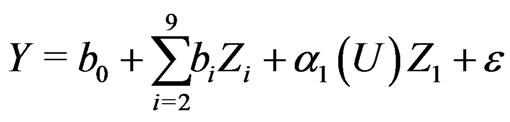 (3.2)
(3.2)
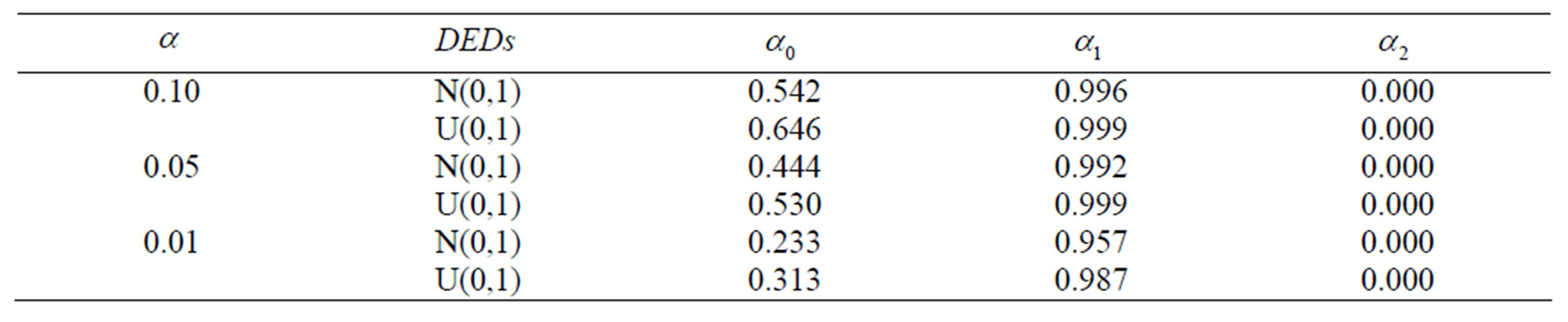
Table 1. Power of the GLR test for  under different error distributions (DEDs) for the CR = 20%.
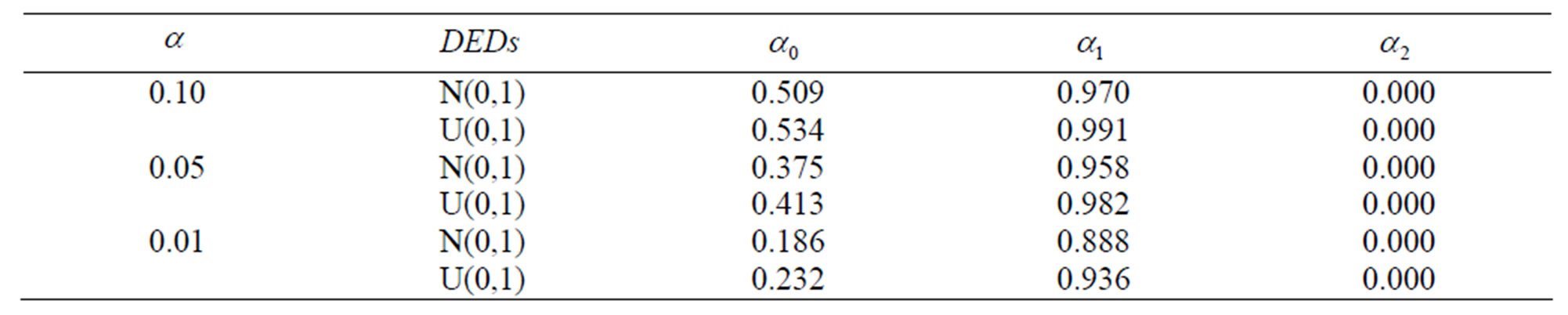
Table 2. Power of the GLR test for  under different error distributions (DEDs) for the CR = 40%.

Table 3. p-values for testing whether a coefficient functions is constant.
And by the method of Fan and Huang (2005), we can estimate the parameters in the model (3.2).
5. References
[1] J. Buckley and I. R. James, "Linear Regression with Censored Data," Biometrika, Vol. 66, No. 3, 1979, pp. 429-436.
[2] Z. Cai, "Trending Time-Varying Coefficient Time Series Models with Serially Correlated Errors," Journal of Econometrics, Vol. 136, No. 1, 2007, pp. 163-188.
[3] K. Chen and X. W. Tong, "Varying Coefficient Transformation Models with Censored Data," Biometrika, Vol. 97, No. 4, 2010, pp. 969-976.
[4] D. M. Dabrowska, "Non-parametric Regression with Censored Survival Time Data," Scandinavian Journal of Statistics, Vol. 14, No. 3, 1987, pp. 181-197.
[5] J. Fan and I. Gijbels, "Censored Regression: Local Linear Approximations and Their Applications," Journal of the American Statistical Association, Vol. 89, No. 426, 1994, pp. 560-570.
[6] J. Fan and T. Huang, "Profile Likelihood Inferences on Semiparametric Varying-Coefficient Partially Linear Models," Bernolli, Vol. 11, No. 6, 2005, pp. 1031-1057.
[7] J. Fan, C. Zhang and J. Zhang, "Generalized Likelihood Ratio Statistics and Wilks Phenomenon," The Annals of Statistics, Vol. 29, No. 1, 2001, pp. 153-193.
[8] J. Fan and W. Zhang, "Statistical Estimation in Varying Coefficient Models," The Annals of Statistics, Vol. 27, No. 5, 1999, pp. 1491-1518.
[9] J. Fan and J. Zhang, "Two-Step Estimation of Functional Linear Models with Application to Longitudinal Data," Journal of Royal Statistical Association B, Vol. 62, No. 2, 2000, pp. 303-322.
[10] H. Wang and Y. Xia, "Shrinkage Estimation of The Varying Coefficient Model," Journal of the American Statistical Association, Vol. 104, No. 486, 2009, pp. 747-757.
[11] T. Hastie and R. Tibshirani, "Varying-Coefficient Models," Journal of Royal Statistical Association B, Vol. 55, No. 4, 1993, pp. 757-796.
[12] H. Koul, V. Susarla and J. Van Ryzin, "Regression Analysis with Randomly Right Censored Data," The Annals of Statistics, Vol. 9, No. 6, 1981, pp. 1276-1288.
[13] S. Leurgans, "Linear Models, Random Censoring and Synthetic Data," Biometrika, Vol. 74, No. 2, 1987, pp. 301-309.
[14] X. Luo, Z. Yang and Y. Zhou, "Varying-Coefficient Regression Models with Censored Data," Acta Mathematicae Applicatae Sinica, Vol. 29, No. 3, 2006, pp. 415-427.
[15] Z. Zheng, "A Class of Estimators of the Parameters in Linear Regression with Censored Data," Acta Mathematicae Applicatae Sinica, Vol. 3, No. 3, 1987, pp. 231-241.
[16] Z. Zheng, "Strong Consistency of Nonparametric Regression Estimates with Censored Data," Journal of Mathematical Research and Exposition, Vol. 8, No. 4, 1988, pp. 307-313.
[17] Y. Zhou and H. Liang, "Statistical Inference for Semiparametric Varying-Coefficient Partially Linear Models with Error-Prone Linear Covariates," The Annals of Statistics, Vol. 37, No. 1, 2009, pp. 427-458.
Appendix
To derive the asymptotic distribution of  under
under , we need the following conditions.
C1. The marginal density  of
of  is Lipschitz continuous and bounded away from 0.
  has a bounded support
 .
.
C2.  has the continuous second derivative.
C3. The function  is symmetric and bounded. Further, the function
  and
and  are bounded and
 .
.
C4. .
.
C5. X is bounded and the  matrix
  is invertible for each
 .
.  and
and  are both Lipschitz continuous.
Remark Conditions (C1)-(C5) are standard conditions, which are commonly used in varyingcoefficient regression model (see Fan, J. and Huang T, 2005 and Luo et al 2006).
Lemma 1. Suppose that  is positive and continuous on a compact interval
 , and
, and  such that
 . Then,
 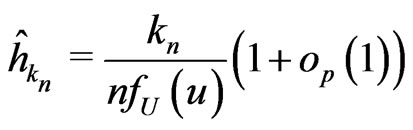 uniformly in
 .
.
Proof. This can be shown by the proof of Theorem 5.1. in Fan and Gijbels (1994).
Lemma 2. Let  be the local linear estimator defined in section 2. Then, under condition (C1)-(C5), uniformly for
 ,
,

where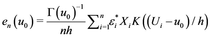 ,
,  with
with .
.
Proof. This follows immediately from the result obtained by Luo et al (2006).
Proof of Theorem 1. Let  denote a generic constant. Then, under
 ,
,
where ,
,  is the design matrix with the
  th row
 and
and  is the projection matrix of
  and
and
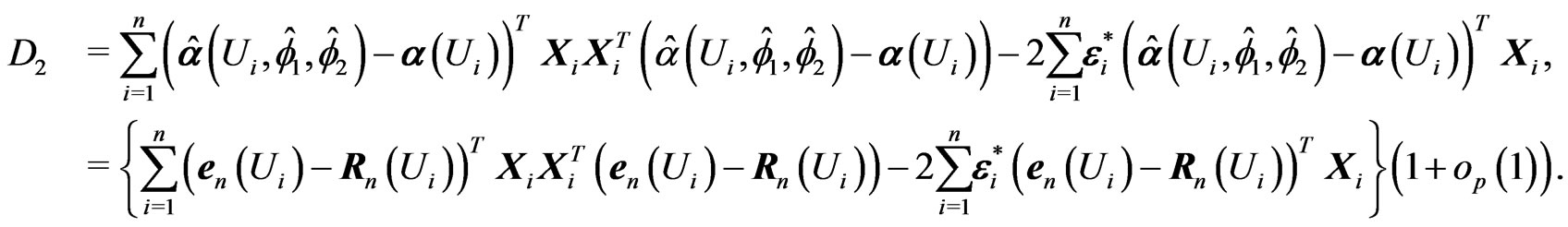
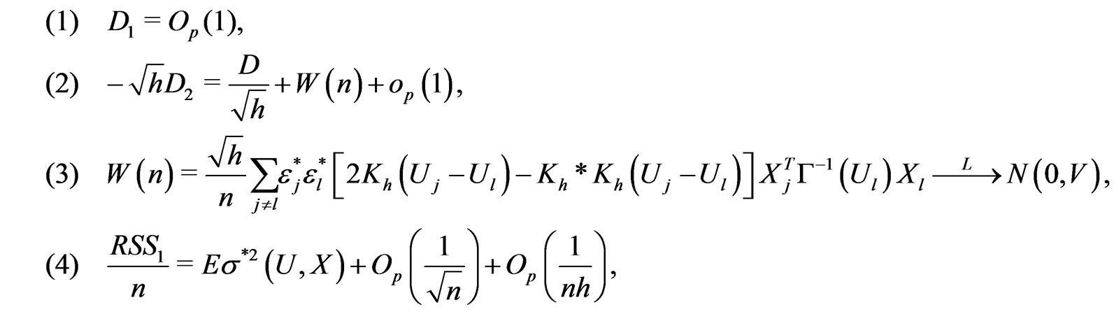
The proof will be completed by showing the following four step.
with
It follows from Lemma 7.1 in Fan et al(2001) that

which implies (1). The proofs of (2) and (3) are the same as the proof of Theorem 5 in Fan et al (2001). The details are omitted. The last step follows from .
.