Open Journal of Statistics
Vol.1 No.1(2011), Article ID:4697,14 pages DOI:10.4236/ojs.2011.11001
Modified Cp Criterion for Optimizing Ridge and Smooth Parameters in the MGR Estimator for the Nonparametric GMANOVA Model
Department of Mathematics, Graduate School of Science, Hiroshima University
1-3-1 Kagamiyama, Higashi-Hiroshima, Hiroshima 739-8626, Japan
E-mail: d093481@hiroshima-u.ac.jp
Shrinkage estimator, Varying coefficient model
Received March 18, 2011; revised April 2, 2011; accepted April 12, 2011
Keywords: Generalized ridge regression, GMANOVA model, Mallows'  statistic, Non-iterative estimator,
Abstract
Longitudinal trends of observations can be estimated using the generalized multivariate analysis of variance (GMANOVA) model proposed by [10]. In the present paper, we consider estimating the trends nonparametrically using known basis functions. Then, as in nonparametric regression, an overfitting problem occurs. [13] showed that the GMANOVA model is equivalent to the varying coefficient model with non-longitudinal covariates. Hence, as in the case of the ordinary linear regression model, when the number of covariates becomes large, the estimator of the varying coefficient becomes unstable. In the present paper, we avoid the overfitting problem and the instability problem by applying the concept behind penalized smoothing spline regression and multivariate generalized ridge regression. In addition, we propose two criteria to optimize hyper parameters, namely, a smoothing parameter and ridge parameters. Finally, we compare the ordinary least square estimator and the new estimator.
1. Introduction
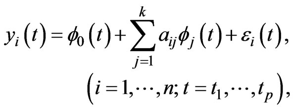
We consider the generalized multivariate analysis of variance (GMANOVA) model with observations of
  -dimensional vectors of response variables. This model was proposed by [10]. Let
 ,
,  ,
,  and
and  be an
be an  matrix of response variables, an
  matrix of non-stochastic centerized between-individual explanatory variables (i.e.,
 )
)
of
 , a
, a  matrix of non-stochastic within-individual explanatory variables of
 , and an
  matrix of error variables, respectively, where
 is the sample size,
  is an
is an  -dimensional vector of ones and
  is a
is a  -dimensional vector of zeros. Then, the GMANOVA model is expressed as
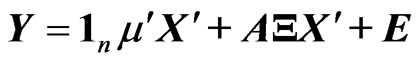
where  is a
is a  unknown regression coefficient matrix an
  is
is  -dimensional unknown vector. We assume that
  where
where  is a
is a  unknown covariance matrix of
 . Then we can express the GMANOVA model as
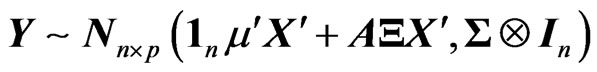
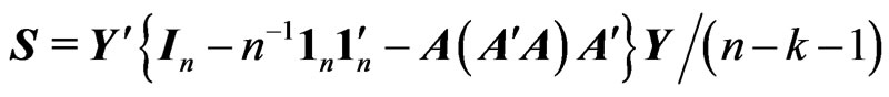
Let  be an unbiased estimator of the unknown covariance matrix
  that is given by
Then, the maximum likelihood (ML) estimators of  and
and are given by
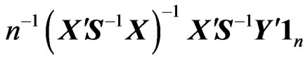 and
and , respectively. The ML estimators are the unbiased and asymptotically efficiency estimators of
  and
and .
.
In the GMANOVA model,  ,
,  is often used as the
  th row vector of
 . Then, we estimate the longitudinal trends of
  using
using  -polynomial curves. However, occasionally, the polynomial curve cannot thoroughly express flexible longitudinal trends. Hence, we consider estimating the longitudinal trends nonparametrically in the same manner as [11] and [5], i.e., we use the known basis function as
  and assume that
  is large. In the present paper, we refer to the GMANOVA model with
  obtained from the basis function as the nonparametric GMANOVA model. In the nonparametric GMANOVA model, it is well known that the ML estimators become unstable because
  becomes unstable when
  is large. Thus, we deal with the least square (LS) estimators of
  and
and , which are obtained by minimizing
 . Then, the LS estimators of
  and
and  are obtained by
  and
and
 respectively. Note that
  does not depend on
 . The LS estimators are simple and unbiased estimators of
  and
and . However, as well as ordinary nonparametric regression model, the LS estimators cause an overfitting problem when we use basis functions to estimate the longitudinal trends nonparametrically. In order to avoid the overfitting problem, we use
  instead of
  as the penalized smoothing spline regression (see, e.g., [2]), where
 is a smoothing parameter and
  is a
is a  known penalty matrix.
Let , and let
 . Then, the GMANOVA model can be expressed as
where  is the
  th element of
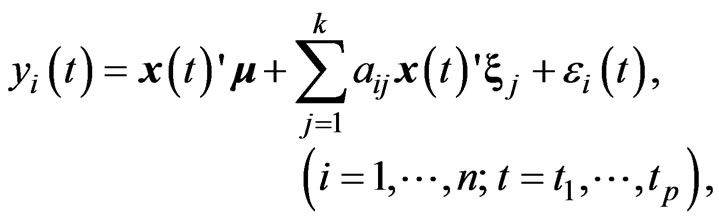
 . This expression indicates that the GMANOVA model is equivalent to the varying coefficient model with non-longitudinal covariates [13], i.e.,
 (4)
(4)
where 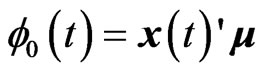 and
and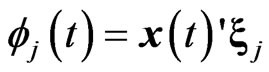 ,
, . Hence, estimating the longitudinal trends in the GMANOVA model nonparametrically is equivalent to estimating the varying coefficients
 ,
,  nonparametrically. However, when multicollinearity occurs in
 , the estimate of
 ,
,  becomes unstable, as does the ordinary LS estimator of regression coefficient, because the variance of an estimator of
  becomes large. Hence, we avoid the multicollinearity problem in
  by the ridge regression.
When  and
and  in the model (1), [4] proposed a ridge regression. This estimator is generally defined by adding
  to
to  in (3), where
  is referred to as a ridge parameter. Since the ridge estimator changes with
 , optimization of
  is very important. One method for optimizing
  is minimizing the
  criterion proposed by [7,8] in the univariate linear regression model (for multivariate case, see e.g., [15]). For the case in which
  and
and , [17] proposed the
  and its bias-corrected
  (modified
 ;
; ) criteria for optimizing the ridge parameter. However, an optimal
  cannot be obtained without an iterative computational algorithm because an optimal
  cannot be obtained in closed form.
On the other hand, [4] also proposed a generalized ridge (GR) regression in the univariate linear regression model, i.e., the model (1) with  and
and , simultaneously with the ridge regression. The GR estimator is defined not by a single ridge parameter, but rather by multiple ridge parameters
 ,
, . Then, several authors proposed a non-iterative GR estimator (see, e.g., [6]). [18] proposed a GR regression in the multivariate linear regression model, i.e., the model (1) with
  and
and . We call this generalized ridge regression the multivariate GR (MGR) regression. They also proposed the
  and
and  criteria for optimizing ridge parameters
  in the MGR regression. They showed that the optimized
  by minimizing two criteria are obtained in closed form. [9] proposed non-iterative MGR estimators by extending non-iterative GR estimators. Several computational tasks are required in estimating
  nonparametrically because we determine the optimal
  and the number of basis functions simultaneously. Fortunately, [18] reported that the performance of the MGR regression is the almost same as that of the multivariate ridge regression. Hence, we use the MGR regression in order to avoid the multicollinearity problem that occurs in
  in order to reduce the number of computational tasks.
The remainder of the present paper is organized as follows: In Section 2, we propose new estimators using the concept of the penalized smoothing spline regression and the MGR regression. In Section 3, we show the target mean squared error (MSE) of a predicted value of . We then propose the
  and
and  criteria to optimize ridge parameters and smoothing parameter in the new estimator. Using these criteria, we show that the optimized ridge parameters are obtained in closed form under the fixed
 . We also show the magnitude relationship between the optimized ridge parameters. In Section 4, we compare the LS estimator in (3) with the proposed estimator through numerical studies. In Section 5, we present our conclusions.
2. The New Estimators
In the model (1), we consider estimating the longitudinal trends nonparametrically by using basis functions . Then, we consider the following estimators in order to avoid the overfitting problem in the nonparametric GMANOVA model,
  and
and
 (5)
(5)
where is a smoothing parameter and
  is a
is a  known penalty matrix. In this estimator, we must determine
  before using this estimator. Since
  is usually set as some nonnegative definite matrix, we assume that
 is a nonnegative definite matrix. If
 , where
 is a
is a  matrix of zeros, then this estimator corresponds to the LS estimators
  and
and  in (1). Note that this estimator controls the smoothness of each estimated curve
  and
and ,
,  through only one parameter
 . When we use this estimator, we need to optimize the parameter
 because this estimator changes with
 .
.
If multicollinearity occurs in , then the LS estimator
  in (1) and the proposed estimator
  in (5) are not good estimators in the sense of having large variance. Note that neither the LS estimator
  nor the proposed estimator
  depend on
 . Hence, we avoid the multicollinearity problem for estimating
 . Multicollinearity often occurs when
  becomes large. Using the following estimator, the multicollinearity problem in
  can be avoided,
 (6)
(6)
where  is a ridge parameter. This estimator with
  corresponds to the estimator of [16]. If
 , then this estimator corresponds to the estimator in (5). Note that
 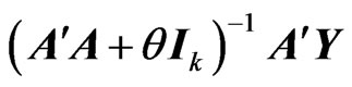 in this estimator corresponds to the ridge estimator for a multivariate linear model [17]. In this estimator, we need to optimize
  and
and  because this estimator changes with these parameters. However, we cannot obtain the optimized
  and
and  in closed form. Thus, we need to use an iterative computational algorithm to optimize two parameters. From another point of view, this estimator controls the smoothness of each estimated curve
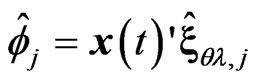 ,
,  through only one parameter
 . Hence, this estimator is not a well fitting curve when the smoothnesses of the true curves differ.
Hence, we apply the concept of the MGR estimator [18] to  in order to obtain the optimized ridge parameter in closed form. Here, we derive the MGR estimator for the nonparametric GMANOVA model as follows:
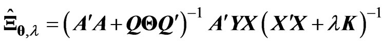 (7)
(7)
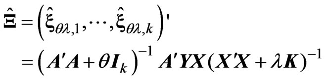
where ,
, is also a ridge parameter,
  , and
, and  is the
  orthogonal matrix that diagonalizes
 , i.e.,
  where
where  and
and 
![]()
![]() are eigenvalues of
are eigenvalues of . It is clearly that
 ,
, . In this estimator, since
  shrinks the estimators of
 ,
,  to 0, we can regard
  as controlling the smoothness of
 . Therefore, in this estimator, rough smoothness of the estimated curves is controlled by
 , and each smoothness of
 ,
,  is controlled by
 .
.
Clearly,  and
and . The
. The  with
with  for some
 corresponds to
  in (6). Thus, the estimator
  includes these estimators. The estimator
  is more flexible than these estimators
  and
and  because
  has
has  parameters and
  or
or  has only one or two parameters. Hence, we consider
  and
and  in estimating the longitudinal trends or the varying coefficient curve, while avoiding the overfitting and multicollinearity problems in the nonparametric GMANOVA model. When
  and
and ,
,  corresponds to the MGR estimator in [18].
3. Main Results
3.1. Target MSE
In order to define the MSE of the predicted value of , we prepare the following discrepancy function for measuring the distance between
  matrices
  and
and
 :
:
Since  is an unknown covariance matrix, we use the unbiased estimator
  in (2) instead of
  to estimate
 . Hence, we estimate
  using the following sample discrepancy function:
 (8)
(8)
These two functions,  and
and , correspond to the summation of the Mahalanobis distance and the sample Mahalanobis distance between the rows of
  and
and , respectively. Clearly,
 and
and . Through simple calculation, we obtain the following properties:
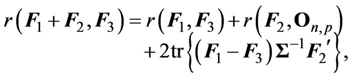
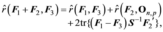
for any  matrices
 ,
,  and
and , Using the discrepancy function
 , the MSE of the predicted value of
  is defined as
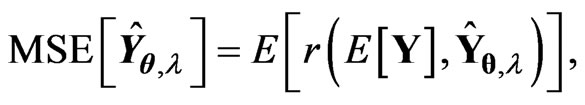 (9)
(9)
where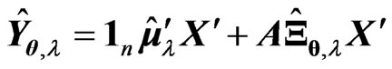 , which is the predicted value of
  when we use
  and
and  in (7). In the present paper, we regard
  and
and  making the MSE the smallest as the principle optimum. However, we cannot use the MSE in (9) in actual application because this MSE includes unknown parameters. Hence, we must estimate (9) in order to estimate the optimum
  and
and .
.
3.2. The  and
and  Criteria
Let and
and . Note that
 . Hence, we obtain
From the properties of the function and using
 , since
  is a nonstochastic variable and
 , and
, and  for any square matrix
 , we obtain
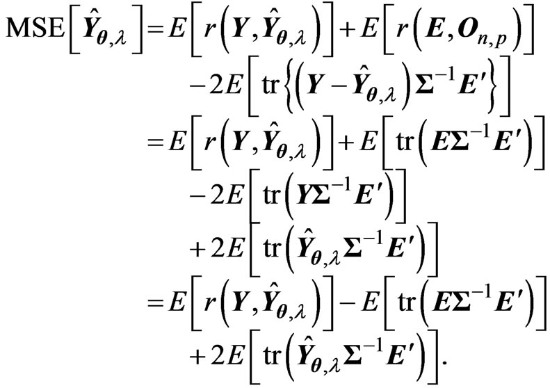
Note that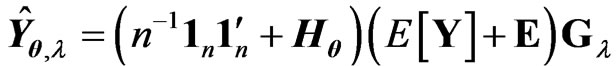 .Thus, we can calculate
  as follows:
because ,
,  and
and  are non-stochastic variables. For calculating the expectations in the MSE, we prove the following lemma.
Lemma 3.1. For any  non-stochastic matrix
 , we obtain
 .
.
proof. Since , we obtain the
  th element of
  as
as ,
, 
 . We obtain
 because
 for any
  and
and  for any
 , where
  is defined as
  if
if  and
and  if
if . Hence we obtain
 . This result means that
  if
if  and
and  if
if . Thus, the lemma is proven.
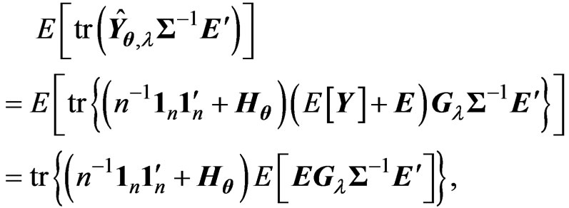
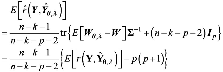
Using this lemma, we obtain 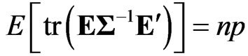 and
and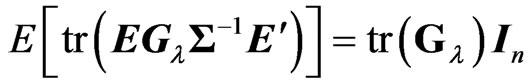 . Hence, we obtain
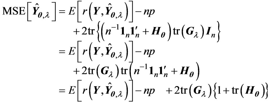
By replacing  with
with , we can propose the instinctive estimator of MSE, referred to as the
  criterion, as follows:
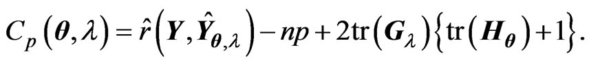 (10)
(10)
When we use this criterion, we optimize the ridge parameter  and the smoothing parameter
  by the following algorithm:
1) We obtain , where
 if
if  is given.
2) We obtain .
.
3) We obtain , where
 ,
, under fixed
 .
.
4) We optimize the ridge parameter and the smoothing parameter as  and
and , respectively.
Note that this  criterion corresponds to that in [18] when
  and
and .
.
There is some bias between the MSE in (9) and the  criterion in (10) because the
  criterion is obtained by replacing
 in the MSE with
 . Generally, when the sample size
  is small or the number of explanatory variables
  is large, this bias becomes large. Then, we cannot obtain the higher-accuracy estimation of the optimum parameters because we cannot obtain the higher-accuracy estimation of MSE of
  in (9). Hence, we correct the bias between
  and the
  criterion. To correct the bias, we assume
 .
.
Let and
and .
.
Note that and
and
 because
  and
and . Then, we obtain Since
 ,
,
 (see, e.g., [14]) and
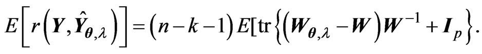
 , we obtain
Therefore, we obtain the unbiased estimator for  as
as , where
 . This implies that the bias corrected
 criterion, denoted as
  (modified
 ) criterion, is obtained by
 (11)
(11)
As in the case of using the , we optimize
  and
and  using this criterion as follows:
1) We obtain , where
 ,
,
 if
if  is given.
2) We obtain .
.
3) We obtain , where
 ,
,  under fixed
 .
.
4) We optimize the ridge parameter and the smoothing parameter as  and
and  , respectively.
Note that the  criterion corresponds to that in [18] when
  and
and . The
. The  criterion completely omits the bias between the MSE of
  in (9) and the
  criterion in (10) by using a number of constant terms
 and
and . If
. If  and
and  can be expressed in closed form for any fixed
 , we do not need the above iterative computational algorithm.
3.3. Optimizations using the  and
and Criteria
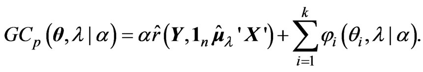
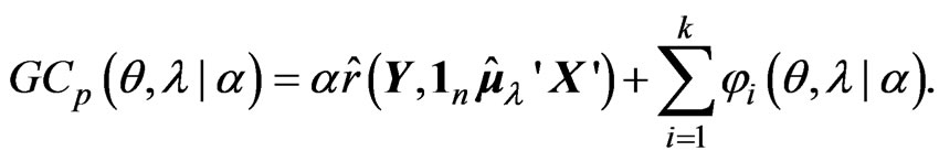
Using the generalized
 criterion, which is given in (14), we can express the
  and
and  criteria as follows:
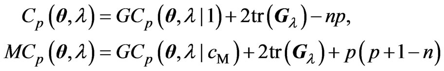
Note that the terms with respect to  in the
  and
and  criteria correspond to
 and
and , respectively. Hence, we consider obtaining the optimum
  by minimizing the
  criterion. From Theorem A, the optimum
  is obtained in closed form as (15). Using the closed form in (15), we obtain
  and
and  for each
  and any fixed
  as follows:
 (12)
(12)
 (13)
(13)
where and
and are the
 th elements of
![]() and
and![]() ,respectively,
,respectively, and
and . Note that
  and
and  vary with
 . Since
  and
and  are regarded as a function of
 , we can regard the
  and
and  criteria for optimizing
  and
and  in (10) and (11) as a function of
 . This means that we can use these criteria to optimize
 .
.
Then, we can rewrite the optimization algorithms to optimize the ridge parameter  and the smoothing parameter
 by minimizing the
  and
and  criteria in (10) and (11) as follows:
1) We obtain and
and .
.
2) We optimize the ridge parameter and the smoothing parameter as  and
and , respectively, by using
 ,
,  and the closed forms in (12) and (13).
This means that we can reduce the processing time to optimize the parameters, and we need to use the optimization algorithm for only one parameter,  , for any
 .
.
3.4. Magnitude Relationships between
Optimized Ridge Parameters
In this subsection, we prove the magnitude relationships between  and
and ,
, .
.
Lemma 3.2. For any , we obtain
 .
.
proof. Since we assume  as a nonnegative definite matrix, there exists
  that satisfies
  (see, e.g., [3]). Then, since
 , we have
 . Hence,
  is a nonnegative definite matrix. This means that all of the eigenvalues of
  are nonnegative. Hence, all of the eigenvalues of
  are nonnegative. Thus,
  is also a nonnegative definite matrix for any
 . Since
 , we obtain
  as a nonnegative definite matrix for any
 . Thus, the lemma is proven.
Using the same idea, we have  for any
 ,
, . Therefore, the final terms of the
  and
and  criteria in (10) and (11) are always greater than
 . In order to prove the magnitude relationship between
  and
and , we consider two situations in which
  is satisfied and
  is satisfied.
First, we consider  to be satisfied. Let
 . Using
 , we obtain the following corollary:
Corollary 3.1. For any , we obtain
 .
.
proof. Through simple calculation, we obtain
Since ,
,  and
and  from lemma 3.1, the corollary is proven.
This corollary indicates that  is satisfied when
  is satisfied because
 , and
, and  is satisfied when
  is satisfied because
  and
and . Using these relationships, we obtain the following theorem.
Theorem 3.1. For any , we obtain
 .
.
proof. We consider the following situations:
1)  is satisfied
2)  is satisfied
3)  is satisfied.
In (1),  , because
 . In (3),
  , because
  becomes
 . Hence, we only consider situation (2). Note that
 , because
  and
and . This means that
  does not become
 . This theorem holds when
 , because, in this case,
  and
and . We also consider
  to be satisfied. Then, we obtain
Since  is a positive definite matrix,
  for any
 . From corollary 3.1, we have
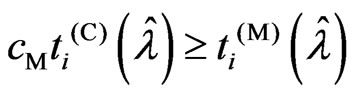 for any
 . Hence we obtain
 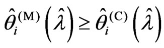 for any
 since
since ,
,  and
and . Thus, this theorem is proven.
This theorem corresponds to that in [9] when  and
and .
.
From Theorem 3.1, we obtained the relationships between  and
and  for the case in which the optimized smoothing parameters
  and
and  are the same. However,
  and
and  are optimized by minimizing the
  and
and  criteria in (10) and (11). Hence,
  and
and  are generally different. Thus, we consider the relationship between
 and
and  when
when . Since
  is regarded as a function of
 , we write
  as
as  and
and  for each optimized smoothing parameter.
Theorem 3.2. We consider the following situations:
1)  or
or  is satisfied
2) and
and are satisfied
3)  is satisfied
4)  is satisfied
5)  or
or is satisfied.
For any  and
and , we obtain the following relationships based on the above situations:
1) If (1), then
2) If (2) and (3), then
3) If (2) and (4), then
4) If (5), then .
.
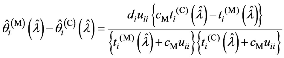
proof. In (1) and (5), the relationships (i) and (iv) are true. Hence we need only prove relationships (ii) and (iii). Then we obtain  and
and  using the closed forms of (12) and (13). Through simple calculation, we obtain Since
  and the denominator is positive, the sign of
  is the same as the sign of
 . Hence we obtain relationships (ii) and (iii). Thus, the theorem is proven.
4. Numerical Studies
In this section, we compare the LS estimator  and
and  in (3) with the proposed estimator
  and
and  in (7) through a numerical study. Let
 , and let
  be an
be an  matrix as follows:
The explanatory matrix  is given by
  where
where ,
,  is an
is an  matrix and each row vector of
  is generated from the independent
  -dimensional normal distribution with mean
  and covariance matrix
 . Let
. Let ,
,  be a
be a  -dimensional vector. We set each
  as follows:
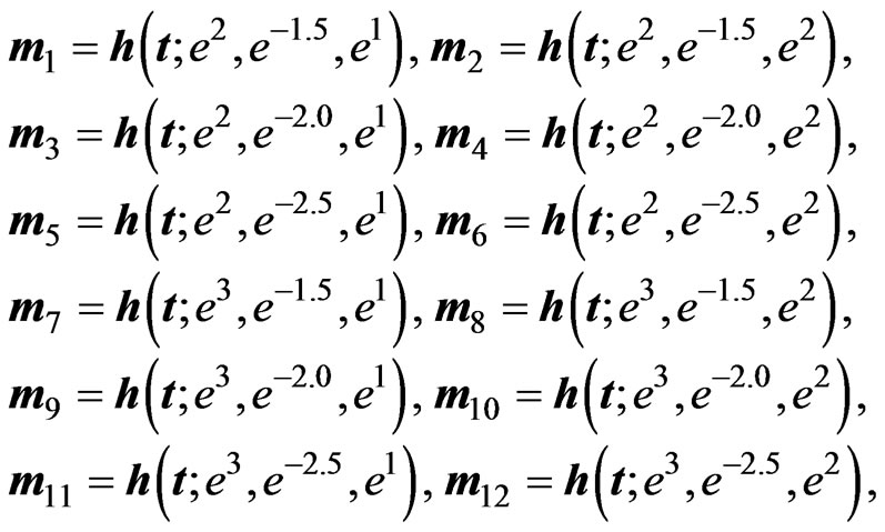
where  and the
 th element of
  is
is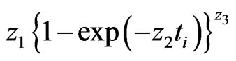 . Each element of
  is Richard's growth curve model [12]. We set the longitudinal trends using these
  as
as . Note that
 ,
, , which indicates that the last six rows of
 are obtained by changing the scale of
 . The response matrix
  is generated by
  where
where . Then, we standardized
 . Let
. Let ,
, and
and . We set each element of
  as a cubic
  -spline basis function. Since
  is set using the cubic
  -spline, we note that
 . Additional details concerning
  and
and  are reported in [2]. We simulate
  repetitions for each
 ,
,  ,
,  ,
,  and
and . In each repetition, we fixed
 , but
, but  varies. We search
 and
and using fminsearch, which is a program in the software Matlab used to search for a minimum value, because
  and
and  cannot be obtained in closed form. In searching
  and
and , we transform
 and search optimized
 by each criterion because
 and
and . In the search algorithm, the starting point for the search is set as
 . Then, we obtain the optimized ridge parameters
  and
and using the closed forms of (12) and (13) in each repetition. In each repetition, we need to optimize
 because
 and
and vary with
 . We calculate
 and
and for each
  in each repetition. Then, we adopt the optimized
  by minimizing each criterion in each repetition. After that, we calculate for
 each criterion, where
 , which is obtained using
  and
and  for each criterion and the optimized
  in each repetition. The average of
  over
over  repetitions is regarded as the MSE of
 . We compare the values predictedusing the estimators
  and
and  with those using the LS estimators
  and
and , and the estimators
  and
and  in (5). When we use
 , we obtain
  by minimizing
  and
and . As in the case of using
 , we adopt
  by using each criterion in each repetition for
  and
and . Some of the results are shown in Tables 1 and 2. The values in the tables are obtained by
 ,
,
 where
where ,and
,and
 where
where .
.
Each estimator optimized by using the  criterion for
 ,
,  , and
, and  is more improve than that by using the
  criterion for each estimator in almost all situations. This indicates that the
  criterion is a better estimator of the MSE of each predicted value of
  than the
  criterion. The reasons for this are that the
  criterion is an unbiased estimator of MSE
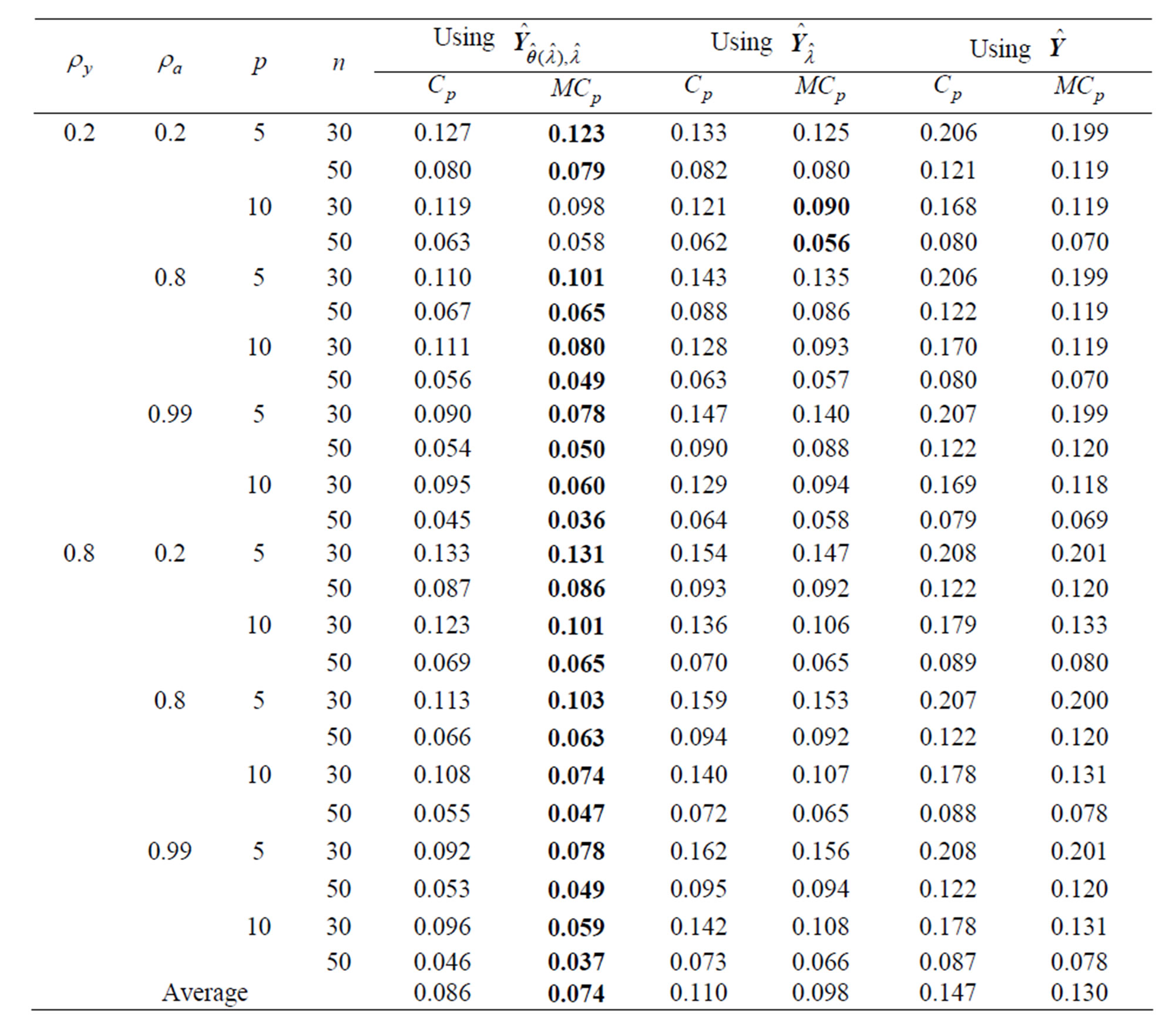
Table 1. MSE when is selected using each criterion for each method in each repetition
 .
.
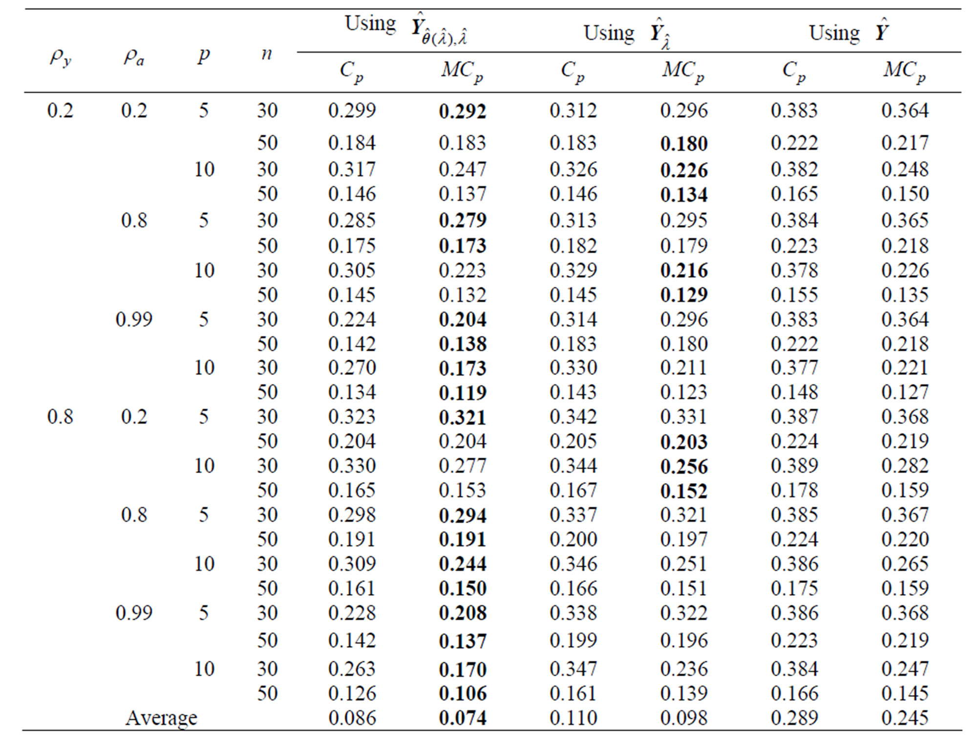
Table 2. MSE when is selected using each criterion for each method in each repetition
 .
.
and each of the parameters in each estimator is optimized by minimizing the  criterion. When
 ,
,  provides a greater improvement than either
  or
or  in all situations. The estimator
 , which is optimized using the
  criterion, has the smallest MSE among these estimators for almost situations when
 . Here,
  provides a greater improvement than
  when
when  in all situations. When
  is large, the estimator
  provides a greater improvement than
  in most situations when
 . On the other hand,
  provides a greater improvement than
  in most situations when
  is small,
  and
and . If
. If , then
  and
and  improve the LS estimator. Comparing the results for
  with the results for
  reveals that these estimators become poor esti mators when
  becomes large. The reasons for this are thought to be that
  and
and  become unstable and the
  has some curves that are in a different scale. Each MSE using each method and the
  criterion is similar to that using the
  criterion if
  becomes large because
  is close to 1. When
  becomes large,
  improves the LS estimator more than when
  is small. Since
  controls the correlation in
 , the multicollinearity in
  becomes large when
  becomes large. Then,
  is not a good estimator because
  is unstable. Hence, we can avoid the multicollinearity problem in
  by using
 , which is one of the purposes of the present study. In all situations, the new estimators improve the LS estimator
 . In addition,
  is better than
  in most situations, especially when
  is small or
  is large. In general,
  optimized using
  is the best method.
5. Conclusions
In the present paper, we estimate the longitudinal trends nonparametrically by using the nonparametric GMANOVA model in (1), which is defined using basis functions as  in the GMANOVA model. When we use basis functions as
 , the LS estimators
  and
and  incur overfitting. In order to avoid this problem, we proposed
  and
and  in (5) using the smoothing parameter
 and the
  known penalty non-negative definite matrix
 . However, if multicollinearity occurs in
 ,
,  and
and  are not good estimators due to large variance. In the present paper, we also proposed
  in (7) in order to avoid the multicollinearity problem that occurs in
  and the overfitting problem by using basis functions as
 . The estimator
  controls the smoothness of each estimated longitudinal curve using only one parameter
 . On the other hand, in the estimator
 , the rough smoothness of estimated longitudinal curves is controlled using
 , and each smoothness of
 in the varying coefficient model (4) is controlled by
 .
.
We also proposed the  and
and  criteria in (10) and (11) for optimizing the ridge parameter
  and the smoothing parameter
 . Then, using the
  criterion in (14) and minimizing this criterion in Theorem A, we obtain the optimized
  using the
  and
and  criteria in closed form as (12) and (13) for any
 . Thus, we can regard the
  and
and  criteria as a function of
 .
.
Hence, we need to optimize only one parameter  in order to optimize
  parameters in
  using these criteria. On the other hand, we must optimize two parameters when we use
  in (6). This optimization is difficult and requires a complicated program and a long processing time for simulation or analysis of real data because the optimized
  cannot be obtained in closed form even if
  is fixed. This is the advantage of using
 . This advantage does not appear to be important because of the high calculation power of CPUs. However, this advantage is made clear when we use
  together with variable selection. Even if
  becomes large, then this advantage remains when
  is used because the optimized
  obtained using each criterion is always obtained as (12) and (13) for any
 . Furthermore, we must optimize
  if we use model (1) to estimate the longitudinal trends. This means that we optimize the parameters in the estimators and calculate the valuation of the estimator for each
 , and then we compare these values in order to optimize
 . Since this optimization requires an iterative computational algorithm, we must reduce the processing time for estimating the parameters in the estimator. Hence, the advantage of using
  is very important. This optimized ridge parameter in (12) and (13) corresponds to that in [18] when
  and
and
 .
.
Using some matrix properties, we showed that  and
and  in the
  and
and  criteria are always nonnegative. From
  for any
  in lemma 3.1, we also established the relationship between
  and
and  for any
  in corollary 3.1. Then, in Theorem 3.1, we established the relationship between
  and
and  if
if  and
and  are the same, where
  and
and  are obtained by minimizing the
  and
and  criteria. Note that this relationship corresponds to that in [9] when
  and
and . In Theorem 3.2, we also established the relationships between
  and
and  for the more general case, in which
  and
and  are different. The reason of the relationship in Theorem 3.2 is occurred is that
  and
and  for each
  can be regarded as a function of
 .
.
The numerical results reveal that  and
and  have some following properties. These estimation methods
  and
and  improve the LS estimator in all situations, especially when
  is large. This indicates that the proposed estimators are better than the LS estimator. Even if
  becomes large, we note that
  is stable because we add the ridge parameter to
  in the LS estimator. This result indicates that the multicollinearity problem in
  can be avoided by using the estimator in (7). These estimators can be used to estimate the true longitudinal trends nonparametrically using basis functions as
  without overfitting. The LS estimator and the proposed estimators
  and
and  optimized using the
  criterion provide a greater improvement than the estimators optimized using the
  criterion in most situations. The reason for this is that the
  criterion is the unbiased estimator of MSE of the predicted value of
 . Based on the present numerical study,
  and
and  can be used to estimate the longitudinal trends in most situations. In addition, the
  can be used to optimize the smoothing parameter
  and the number of basis functions
 . Hence, we can use
  and
and , the parameters
 ,
,  , and
, and  of which are optimized by the
  criterion for estimating the longitudinal trends.
6. Acknowledgments
I would like to express my deepest gratitude to Dr. Hirokazu Yanagihara of Hiroshima University for his valuable ideas and useful discussions. In addition, I would like to thank Prof. Yasunori Fujikoshi, Prof. Hirofumi Wakaki, Dr. Kenichi Satoh and Dr. Kengo Kato of Hiroshima University for their useful suggestions and comments. Finally, I would like to thank Dr. Tomoyuki Akita of Hiroshima University for his advice with regard to programming.
7. Appendix
7.1. Minimization of the  Criterion
In this appendix, we show that the optimizations using the  and
and  criteria in (10) and (11) are obtained in closed form as (12) and (13) for any
 . [9] proposed the generalized
 criterion for the MGR regression (originally the
  criterion for selection variables in the univariate regression was proposed by [1]). Similar to their idea, we proposed the
  criterion for the nonparametric GMANOVA model.
By omitting constant terms and some terms with respect to  in the
  and
and  criteria in (10) and (11), these criteria are included in a class of criteria specified by
 . This class is expressed by the
 criterion as
 (14)
(14)
where the function  is given by (8). Note that
  and
and  correspond to the terms with respect to
  in the
  and
and  criteria. Using this
  criterion, we can deal systematically with the
  and
and  criteria for optimizing
 . Let
. Let ,
, which minimize the
  criterion for any
 . Then,
  and
and  are obtained as
 and
and , respectively. Thus, we can deal systematically with the optimizations of
  when we use the
  and
and  criteria. This means that we need only obtain
  in order to obtain
  and
and  for any
 and some
 . If
. If  is obtained in closed form for any fixed
 , we do not need to use the iterative computational algorithm for optimizing the ridge parameter
 . In order to obtain
 , we obtain
 ,
,  in closed form, as shown in the following theorem.
Theorem A. For any  and
and
 ,
,  is obtained as
 (15)
(15)
where .
.
proof. Since 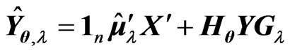 and we use the

properties of the function  in Section 3.1, we can calculate
  in the
  criterion in (14) as follows:
Since for any
 ,
,  and
and  for any
 , the second term in the right-hand side of the above equation can be calculated as Note that
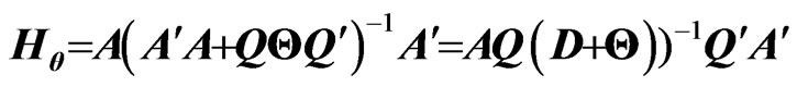 because
  is an orthogonal matrix and
 . Hence, we obtain the following results:

Since  and
and  are diagonal matrices, we obtain
 . Hence
  is calculated as
where and
and . Clearly,
  and
and  change with
 . Based on this result and
 , we can calculate the
  criterion in (14) as follows:

Then, we calculate the second and third terms in the right-hand side of the above equation as follows:
where  and
and  are the
  th element of
  and
and , respectively. Clearly,
  and
and  also vary with
 . Note that
 ,
,  for any
  because
  is a positive definite matrix (see, e.g., [3]). Let
 ,
,  be as follows:
 (16)
(16)
Using , we can express
Since  does not depend on
 , we can obtain
  by minimizing
  for each
  and any
 . In order to obtain
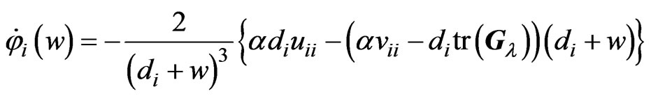
 , we consider the following function for
 :
:
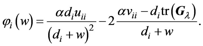 (17)
(17)
If we restrict  to be greater than or equal to 0, then this function is equivalent to the function
  in (16), which must be minimized. Note that
  and
and . Letting
 , we obtain
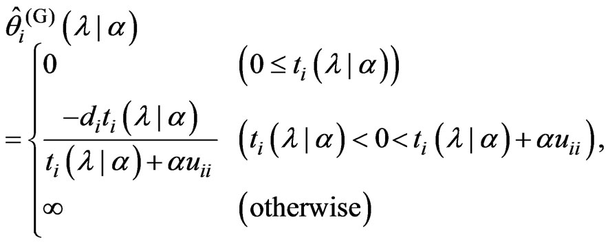
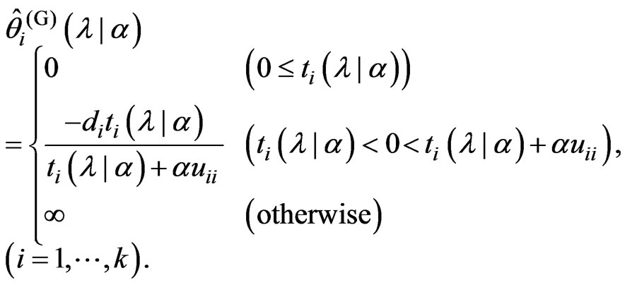
Let  satisfy
  and
and , then
  is obtained by
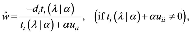
where . Note that
  in (17) has a minimum value at
 , which is
  and
and . Note that the sign of
  is the same as the sign of
 . In order to obtain
 , we consider the following situations:
1)  is satisfied
2)  and
and  are satisfied
3)  and
and  are satisfied.
In (1),  , because
  and
and . In addition,
  for any
 , because
 , and
, and  indicates that the sign of
  is nonnegative. This means that the minimum value of
  in
in  is obtained when
  in situation (1). In (2),
  , and then the minimum value of
  in
in  is obtained when
 . In (3), since
  and
and , we obtain
 for any
 . Hence,
  is minimized when
  in
in . From the above results, we obtain
 as follows:
Thus, the theorem is proven.
Note that  corresponds to that in [9] when
  and
and . Since we obtain
  and
and  in closed form as (15) for any
 , we must optimize only one parameter
  in order to optimize
  parameters. The use of
  is advantageous because only an iterative computational algorithm is required for optimizing only one parameter
  for any
 . This means that we can reduce the processing time required to optimize the parameters in the estimator
  which is defined by (7). When we use
  in (5), we also need the same iterative computational algorithm to optimize only one parameter
 .
.
On the other hand, when we use  in (6), the
  criterion for optimizing
  for any fixed
  is obtained as
Since we need to minimize  in order to optimize
 , we cannot obtain
  that minimizes this
  criterion for
  in closed form, even if
  is fixed. Thus, we use an iterative computational algorithm to optimize the parameters
  and
and  simultaneously. This iterative computational algorithm for optimizing two parameters is difficult and requires a longer processing time than the optimization of a single parameter
8. References
[1] A. C. Atkinson, “A note on the generalized information criterion for choice of a model,” Biometrika, vol. 67, no. 2, March 1980, pp. 413-418., pp. 291-293.
[2] P. J. Green and B. W. Silverman, “Nonparametric Regression and Generalized Linear Models,” Chapman & Hall/CRC, 1994.
[3] D. A. Harville, “Matrix Algebra from a Statistician’s Perspective,” New York Springer, 1997.
[4] A. E. Hoerl and R. W. Kennard, “Ridge regression: biased estimation for nonorthogonal problems,” Technometrics, vol. 12, No. 1, February 1970, pp. 55-67.
[5] A. M. Kshirsagar and W. B. Smith, “Growth Curves,” Marcel Dekker, 1995.
[6] J. F. Lawless, “Mean squared error properties of generalized ridge regression,” Journal of the American Statistical Association, vol. 76, no. 374, 1981, pp. 462-466.
[7] C. L. Mallows, “Some comments on Cp,” Technometrics, vol. 15, no. 1, November 1973, pp. 661-675.
[8] C. L. Mallows, “More comments on Cp,” Technometrics, vol. 37, no. 4, November 1995, pp. 362-372.
[9] I. Nagai, H. Yangihara and K. Satoh, “Optimization of Ridge Parameters in Multivariate Generalized Ridge Regression by Plug-in Methods,” TR 10-03, Statistical Research Group, Hiroshima University, 2010.
[10] R. F. Potthoff and S. N. Roy, “A generalized multivariate analysis of variance model useful especially for growth curve problems,” Biometrika, vol. 51, no. 3–4, December 1964, pp. 313-326.
[11] K. S. Riedel and K. Imre, “Smoothing spline growth curves with covariates,” Communications in Statistics – Theory and Methods, vol. 22, no. 7, 1993, pp. 1795-1818.
[12] F. J. Richard, “A flexible growth function for empirical use,” Journal of Experimental Botany, vol. 10, no. 2, 1959, pp. 290–301.
[13] K. Satoh and H. Yanagihara, “Estimation of varying coefficients for a growth curve model,” American Journal of Mathematical and Management Sciences, 2010 (in press).
[14] M. Siotani, T. Hayakawa and Y. Fujikoshi, “Modern Multivariate Statistical Analysis: A Graduate Course and Handbook,” American Sciences Press, Columbus, Ohio, 1985.
[15] R. S. Sparks, D. Coutsourides and L. Troskie, “The multivariate ,” Communications in Statistics - Theory and Methods, vol. 12, no. 15, 1983, pp. 1775-1793.
[16] Y. Takane, K. Jung and H. Hwang, “Regularized reduced rank growth curve models,” Computational Statistics and Data Analysis, vol. 55, no. 2, February 2011, pp. 1041-1052.
[17] H. Yanagihara and K. Satoh, “An unbiased Cp criterion for multivariate ridge regression,” Journal of Multivariate Analysis, vol. 101, no. 5, May 2010, pp. 1226-1238.
[18] H. Yanagihara, I. Nagai and K. Satoh, “A bias-corrected Cp criterion for optimizing ridge parameters in multivariate generalized ridge regression,” Japanese Journal of Applied Statistics, vol. 38, no. 3, October 2009, pp. 151-172 (in Japanese).