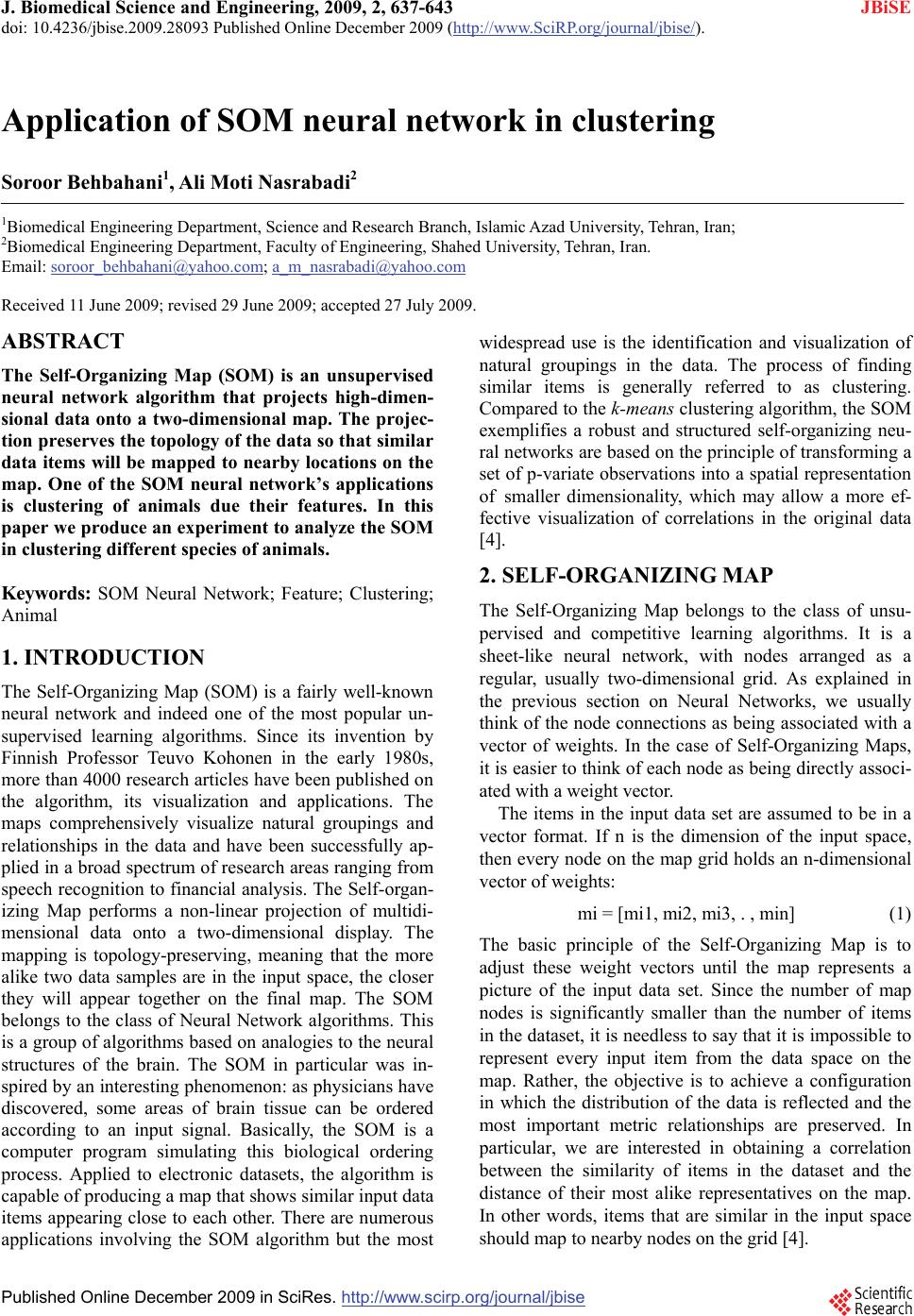J. Biomedical Science and Engineering, 2009, 2, 637-643
doi: 10.4236/jbise.2009.28093 Published Online December 2009 (http://www.SciRP.org/journal/jbise/
JBiSE
).
Published Online December 2009 in SciRes.http://www.scirp.org/journal/jbise
Application of SOM neural network in clustering
Soroor Behbahani1, Ali Moti Nasrabadi2
1Biomedical Engineering Department, Science and Research Branch, Islamic Azad University, Tehran, Iran;
2Biomedical Engineering Department, Faculty of Engineering, Shahed University, Tehran, Iran.
Received 11 June 2009; revised 29 June 2009; accepted 27 July 2009.
ABSTRACT
The Self-Organizing Map (SOM) is an unsupervised
neural network algorithm that projects high-dimen-
sional data onto a two-dimensional map. The projec-
tion preserves the topology of the data so that similar
data items will be mapped to nearby locations on the
map. One of the SOM neural network’s applications
is clustering of animals due their features. In this
paper we produce an experiment to analyze the SOM
in clustering different species of animals.
Keywords: SOM Neural Network; Feature; Clustering;
Animal
1. INTRODUCTION
The Self-Organizing Map (SOM) is a fairly well-known
neural network and indeed one of the most popular un-
supervised learning algorithms. Since its invention by
Finnish Professor Teuvo Kohonen in the early 1980s,
more than 4000 research articles have been published on
the algorithm, its visualization and applications. The
maps comprehensively visualize natural groupings and
relationships in the data and have been successfully ap-
plied in a broad spectrum of research areas ranging from
speech recognition to financial analysis. The Self-organ-
izing Map performs a non-linear projection of multidi-
mensional data onto a two-dimensional display. The
mapping is topology-preserving, meaning that the more
alike two data samples are in the input space, the closer
they will appear together on the final map. The SOM
belongs to the class of Neural Network algorithms. This
is a group of algorithms based on analogies to the neural
structures of the brain. The SOM in particular was in-
spired by an interesting phenomenon: as physicians have
discovered, some areas of brain tissue can be ordered
according to an input signal. Basically, the SOM is a
computer program simulating this biological ordering
process. Applied to electronic datasets, the algorithm is
capable of producing a map that shows similar input data
items appearing close to each other. There are numerous
applications involving the SOM algorithm but the most
widespread use is the identification and visualization of
natural groupings in the data. The process of finding
similar items is generally referred to as clustering.
Compared to the k-means clustering algorithm, the SOM
exemplifies a robust and structured self-organizing neu-
ral networks are based on the principle of transforming a
set of p-variate observations into a spatial representation
of smaller dimensionality, which may allow a more ef-
fective visualization of correlations in the original data
[4].
2. SELF-ORGANIZING MAP
The Self-Organizing Map belongs to the class of unsu-
pervised and competitive learning algorithms. It is a
sheet-like neural network, with nodes arranged as a
regular, usually two-dimensional grid. As explained in
the previous section on Neural Networks, we usually
think of the node connections as being associated with a
vector of weights. In the case of Self-Organizing Maps,
it is easier to think of each node as being directly associ-
ated with a weight vector.
The items in the input data set are assumed to be in a
vector format. If n is the dimension of the input space,
then every node on the map grid holds an n-dimensional
vector of weights:
mi = [mi1, mi2, mi3, . , min] (1)
The basic principle of the Self-Organizing Map is to
adjust these weight vectors until the map represents a
picture of the input data set. Since the number of map
nodes is significantly smaller than the number of items
in the dataset, it is needless to say that it is impossible to
represent every input item from the data space on the
map. Rather, the objective is to achieve a configuration
in which the distribution of the data is reflected and the
most important metric relationships are preserved. In
particular, we are interested in obtaining a correlation
between the similarity of items in the dataset and the
distance of their most alike representatives on the map.
In other words, items that are similar in the input space
should map to nearby nodes on the grid [4].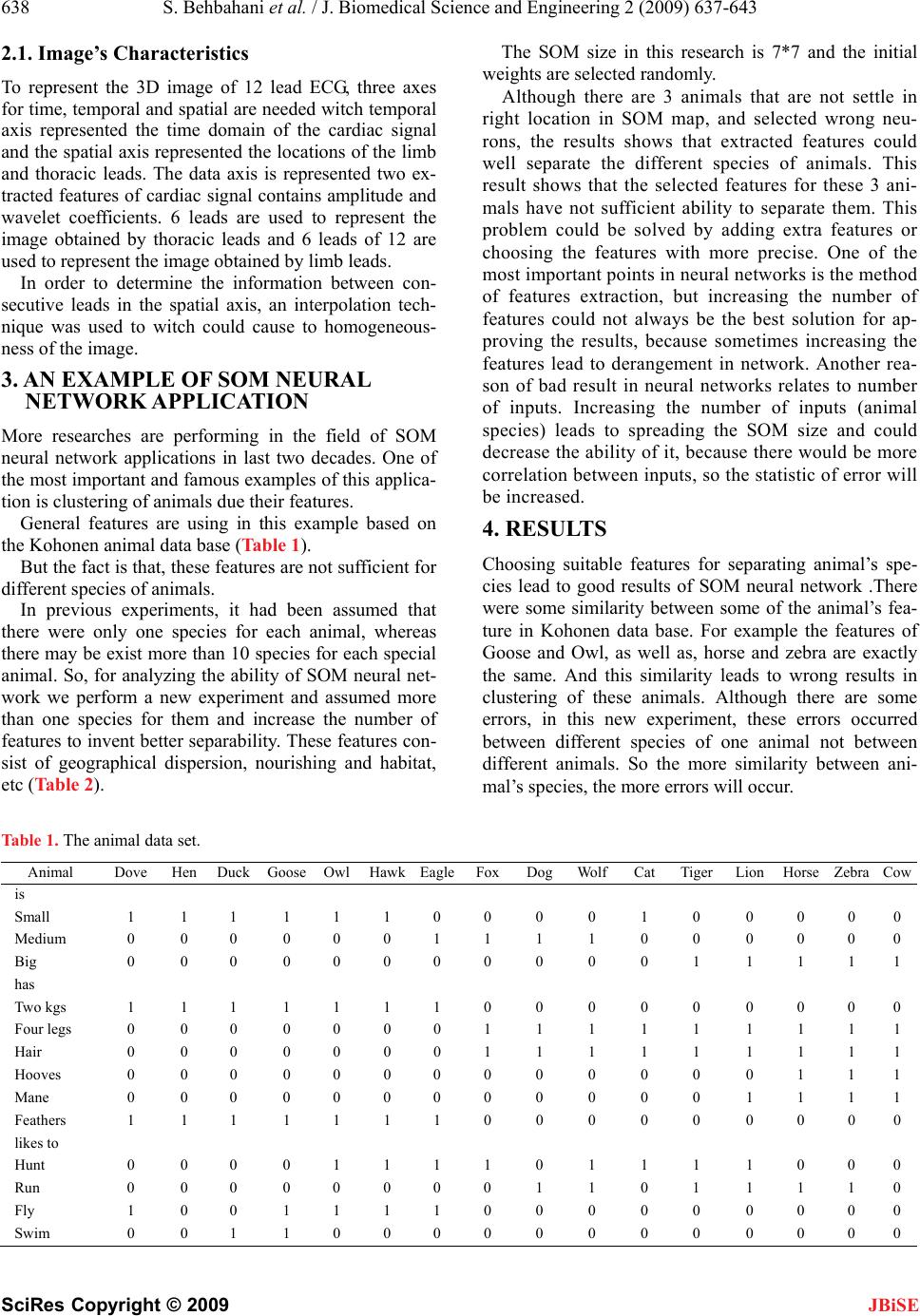

638 S. Behbahani et al. / J. Biomedical Science and Engineering 2 (2009) 637-643
SciRes Copyright © 2009 JBiSE
2.1. Image’s Characteristics
To represent the 3D image of 12 lead ECG, three axes
for time, temporal and spatial are needed witch temporal
axis represented the time domain of the cardiac signal
and the spatial axis represented the locations of the limb
and thoracic leads. The data axis is represented two ex-
tracted features of cardiac signal contains amplitude and
wavelet coefficients. 6 leads are used to represent the
image obtained by thoracic leads and 6 leads of 12 are
used to represent the image obtained by limb leads.
In order to determine the information between con-
secutive leads in the spatial axis, an interpolation tech-
nique was used to witch could cause to homogeneous-
ness of the image.
3. AN EXAMPLE OF SOM NEURAL
NETWORK APPLICATION
More researches are performing in the field of SOM
neural network applications in last two decades. One of
the most important and famous examples of this applica-
tion is clustering of animals due their features.
General features are using in this example based on
the Kohonen animal data base (Table 1).
But the fact is that, these features are not sufficient for
different species of animals.
In previous experiments, it had been assumed that
there were only one species for each animal, whereas
there may be exist more than 10 species for each special
animal. So, for analyzing the ability of SOM neural net-
work we perform a new experiment and assumed more
than one species for them and increase the number of
features to invent better separability. These features con-
sist of geographical dispersion, nourishing and habitat,
etc (Table 2).
The SOM size in this research is 7*7 and the initial
weights are selected randomly.
Although there are 3 animals that are not settle in
right location in SOM map, and selected wrong neu-
rons, the results shows that extracted features could
well separate the different species of animals. This
result shows that the selected features for these 3 ani-
mals have not sufficient ability to separate them. This
problem could be solved by adding extra features or
choosing the features with more precise. One of the
most important points in neural networks is the method
of features extraction, but increasing the number of
features could not always be the best solution for ap-
proving the results, because sometimes increasing the
features lead to derangement in network. Another rea-
son of bad result in neural networks relates to number
of inputs. Increasing the number of inputs (animal
species) leads to spreading the SOM size and could
decrease the ability of it, because there would be more
correlation between inputs, so the statistic of error will
be increased.
4. RESULTS
Choosing suitable features for separating animal’s spe-
cies lead to good results of SOM neural network .There
were some similarity between some of the animal’s fea-
ture in Kohonen data base. For example the features of
Goose and Owl, as well as, horse and zebra are exactly
the same. And this similarity leads to wrong results in
clustering of these animals. Although there are some
errors, in this new experiment, these errors occurred
between different species of one animal not between
different animals. So the more similarity between ani-
mal’s species, the more errors will occur.
Table 1. The animal data set.
Animal Dove Hen Duck Goose Owl HawkEagleFox DogWolfCatTiger Lion Horse ZebraCow
is
Small 1 1 1 1 1 1 0 0 0 0 1 0 0 0 0 0
Medium 0 0 0 0 0 0 1 1 1 1 0 0 0 0 0 0
Big 0 0 0 0 0 0 0 0 0 0 0 1 1 1 1 1
has
Two kgs 1 1 1 1 1 1 1 0 0 0 0 0 0 0 0 0
Four legs 0 0 0 0 0 0 0 1 1 1 1 1 1 1 1 1
Hair 0 0 0 0 0 0 0 1 1 1 1 1 1 1 1 1
Hooves 0 0 0 0 0 0 0 0 0 0 0 0 0 1
1 1
Mane 0 0 0 0 0 0 0 0 0 0 0 0 1 1 1 1
Feathers 1 1 1 1 1 1 1 0 0 0 0 0 0 0 0 0
likes to
Hunt 0 0 0 0 1 1 1 1 0 1 1 1 1 0 0 0
Run 0 0 0 0 0 0 0 0 1 1 0 1 1 1 1 0
Fly 1 0 0 1 1 1 1 0 0 0 0 0 0 0 0 0
Swim 0 0 1 1 0 0 0 0 0 0 0 0 0 0 0 0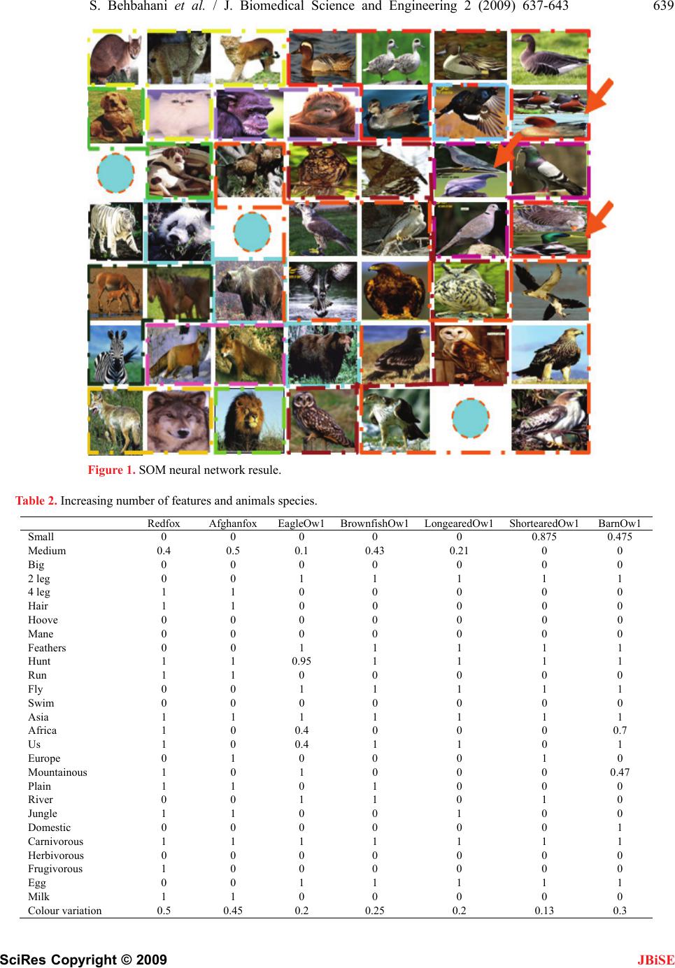

S. Behbahani et al. / J. Biomedical Science and Engineering 2 (2009) 637-643 639
SciRes Copyright © 2009
Figure 1. SOM neural network resule.
Table 2. Increasing number of features and animals species.
Redfox Afghanfox EagleOw1BrownfishOw1LongearedOw1ShortearedOw1 BarnOw1
Small 0 0 0 0 0 0.875 0.475
Medium 0.4 0.5 0.1 0.43 0.21 0 0
Big 0 0 0 0 0 0 0
2 leg 0 0 1 1 1 1 1
4 leg 1 1 0 0 0 0 0
Hair 1 1 0 0 0 0 0
Hoove 0 0 0 0 0 0 0
Mane 0 0 0 0 0 0 0
Feathers 0 0 1 1 1 1 1
Hunt 1 1 0.95 1 1 1 1
Run 1 1 0 0 0 0 0
Fly 0 0 1 1 1 1 1
Swim 0 0 0 0 0 0 0
Asia 1 1 1 1 1 1 1
Africa 1 0 0.4 0 0 0 0.7
Us 1 0 0.4 1 1 0 1
Europe 0 1 0 0 0 1 0
Mountainous 1 0 1 0 0 0 0.47
Plain 1 1 0 1 0 0 0
River 0 0 1 1 0 1 0
Jungle 1 1 0 0 1 0 0
Domestic 0 0 0 0 0 0 1
Carnivorous 1 1 1 1 1 1 1
Herbivorous 0 0 0 0 0 0 0
Frugivorous 1 0 0 0 0 0 0
Egg 0 0 1 1 1 1 1
Milk 1 1 0 0 0 0 0
Colour variation 0.5 0.45 0.2 0.25 0.2 0.13 0.3
JBiSE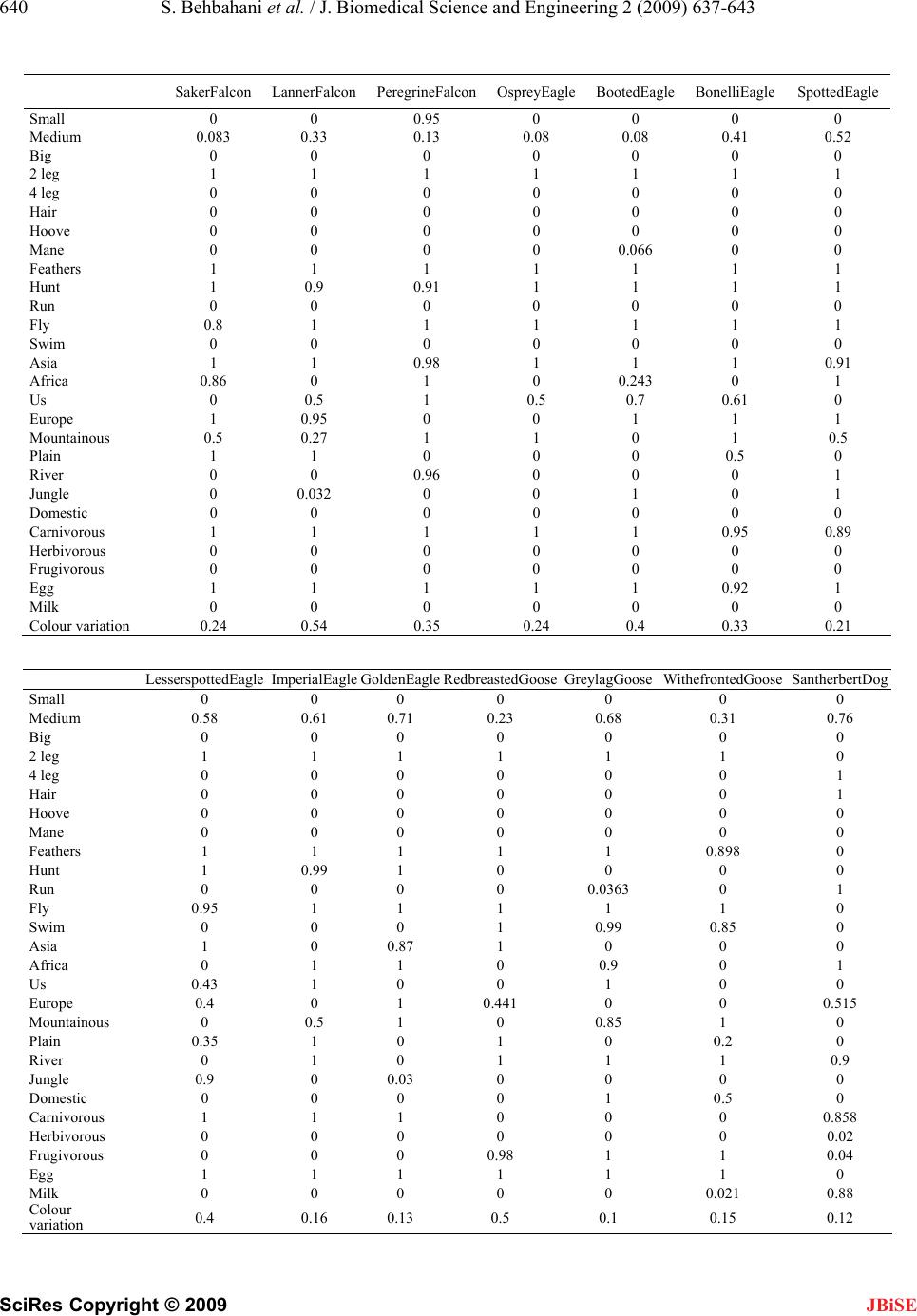

640 S. Behbahani et al. / J. Biomedical Science and Engineering 2 (2009) 637-643
SciRes Copyright © 2009 JBiSE
SakerFalcon LannerFalcon PeregrineFalconOspreyEagleBootedEagleBonelliEagle SpottedEagle
Small 0 0 0.95000 0
Medium 0.083 0.33 0.13 0.08 0.08 0.41 0.52
Big 0 0 0 0 0 0 0
2 leg 1 1 1 1 1 1 1
4 leg 0 0 0 0 0 0 0
Hair 0 0 0 0 0 0 0
Hoove 0 0 0 0 0 0 0
Mane 0 0 0 0 0.066 0 0
Feathers 1 1 1 1 1 1 1
Hunt 1 0.9 0.91 1 1 1 1
Run 0 0 0 0 0 0 0
Fly 0.8 1 1 1 1 1 1
Swim 0 0 0 0 0 0 0
Asia 1 1 0.98 1 1 1 0.91
Africa 0.86 0 1 0 0.243 0 1
Us 0 0.5 1 0.5 0.7 0.61 0
Europe 1 0.95 0 0 1 1 1
Mountainous 0.5 0.27 1 1 0 1 0.5
Plain 1 1 0 0 0 0.5 0
River 0 0 0.96 0 0 0 1
Jungle 0 0.032 0 0 1 0 1
Domestic 0 0 0 0 0 0 0
Carnivorous 1 1 1 1 1 0.95 0.89
Herbivorous 0 0 0 0 0 0 0
Frugivorous 0 0 0 0 0 0 0
Egg 1 1 1 1 1 0.92 1
Milk 0 0 0 0 0 0 0
Colour variation 0.24 0.54 0.35 0.24 0.4 0.33 0.21
LesserspottedEagle ImperialEagle GoldenEagleRedbreastedGooseGreylagGooseWithefrontedGoose SantherbertDog
Small 0 0 0 0 0 0 0
Medium 0.58 0.61 0.71 0.23 0.68 0.31 0.76
Big 0 0 0 0 0 0 0
2 leg 1 1 1 1 1 1 0
4 leg 0 0 0 0 0 0 1
Hair 0 0 0 0 0 0 1
Hoove 0 0 0 0 0 0 0
Mane 0 0 0 0 0 0 0
Feathers 1 1 1 1 1 0.898 0
Hunt 1 0.99 1 0 0 0 0
Run 0 0 0 0 0.0363 0 1
Fly 0.95 1 1 1 1 1 0
Swim 0 0 0 1 0.99 0.85 0
Asia 1 0 0.87 1 0 0 0
Africa 0 1 1 0 0.9 0 1
Us 0.43 1 0 0 1 0 0
Europe 0.4 0 1 0.441 0 0 0.515
Mountainous 0 0.5 1 0 0.85 1 0
Plain 0.35 1 0 1 0 0.2 0
River 0 1 0 1 1 1 0.9
Jungle 0.9 0 0.03 0 0 0 0
Domestic 0 0 0 0 1 0.5 0
Carnivorous 1 1 1 0 0 0 0.858
Herbivorous 0 0 0 0 0 0 0.02
Frugivorous 0 0 0 0.98 1 1 0.04
Egg 1 1 1 1 1 1 0
Milk 0 0 0 0 0 0.021 0.88
Colour
variation 0.4 0.16 0.13 0.5 0.1 0.15 0.12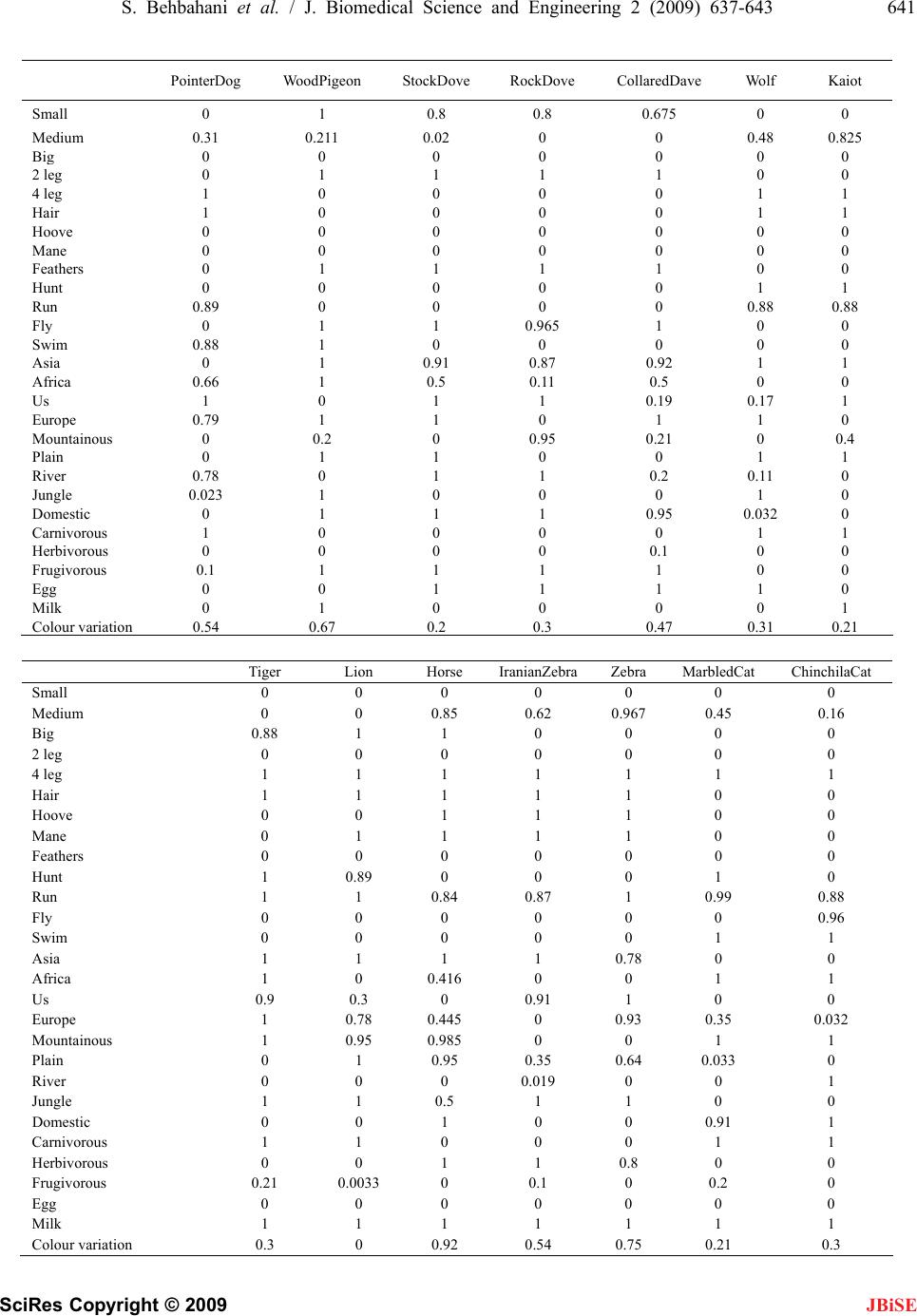

S. Behbahani et al. / J. Biomedical Science and Engineering 2 (2009) 637-643 641
SciRes Copyright © 2009 JBiSE
PointerDog WoodPigeon StockDove RockDove CollaredDave Wolf Kaiot
Small 0 1 0.8 0.8 0.675 0 0
Mediu
m
0.31 0.211 0.020 00.48 0.825
Bi
g
0 0 0000 0
2 le
g
0 1 1110 0
4 le
g
1 0 0001 1
Hai
r
1 0 0001 1
Hoove 0 0 0000 0
Mane 0 0 0000 0
Feathers 0 1 1110 0
Hun
t
0 0 0001 1
Run 0.89 0 0000.88 0.88
Fl
y
0 1 10.96510 0
Swi
m
0.88 1 0000 0
Asia 0 1 0.910.870.921 1
Africa 0.66 1 0.50.110.50 0
Us 1 0 110.190.17 1
Euro
p
e 0.79 1 1011 0
Mountainous 0 0.2 0 0.95 0.210 0.4
Plain 0 1 1001 1
Rive
r
0.78 0 110.20.11 0
Jun
g
le 0.023 1 0001 0
Domestic 0 1 110.950.032 0
Carnivorous 1 0 0001 1
Herbivorous 0 0 000.10 0
Fru
g
ivorous 0.1 1 1110 0
E
gg
0 0 1111 0
Mil
k
0 1 0000 1
Colour variation 0.54 0.67 0.20.30.470.31 0.21
Tiger Lion Horse IranianZebraZebra MarbledCat ChinchilaCat
Small 0 0 0 0 0 0 0
Medium 0 0 0.85 0.62 0.967 0.45 0.16
Big 0.88 1 1 0 0 0 0
2 leg 0 0 0 0 0 0 0
4 leg 1 1 1 1 1 1 1
Hair 1 1 1 1 1 0 0
Hoove 0 0 1 1 1 0 0
Mane 0 1 1 1 1 0 0
Feathers 0 0 0 0 0 0 0
Hunt 1 0.89 0 0 0 1 0
Run 1 1 0.84 0.87 1 0.99 0.88
Fly 0 0 0 0 0 0 0.96
Swim 0 0 0 0 0 1 1
Asia 1 1 1 1 0.78 0 0
Africa 1 0 0.416 0 0 1 1
Us 0.9 0.3 0 0.91 1 0 0
Europe 1 0.78 0.445 0 0.93 0.35 0.032
Mountainous 1 0.95 0.985 0 0 1 1
Plain 0 1 0.95 0.35 0.64 0.033 0
River 0 0 0 0.019 0 0 1
Jungle 1 1 0.5 1 1 0 0
Domestic 0 0 1 0 0 0.91 1
Carnivorous 1 1 0 0 0 1 1
Herbivorous 0 0 1 1 0.8 0 0
Frugivorous 0.21 0.0033 0 0.1 0 0.2 0
Egg 0 0 0 0 0 0 0
Milk 1 1 1 1 1 1 1
Colour variation 0.3 0 0.92 0.54 0.75 0.21 0.3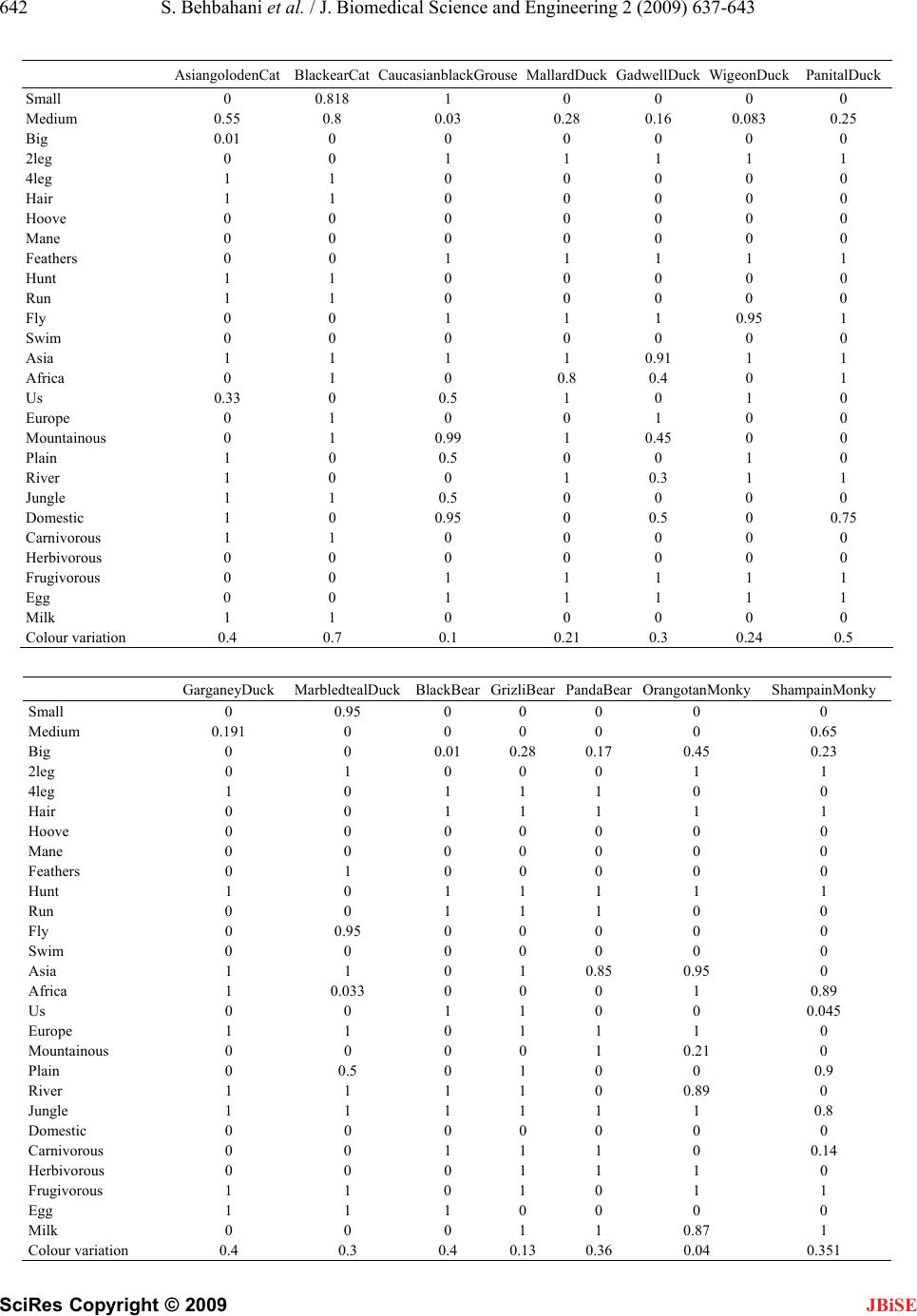

642 S. Behbahani et al. / J. Biomedical Science and Engineering 2 (2009) 637-643
SciRes Copyright © 2009 JBiSE
AsiangolodenCat BlackearCatCaucasianblackGrouseMallardDuck GadwellDuck WigeonDuck PanitalDuck
Small 0 0.818 1 0 0 0 0
Medium 0.55 0.8 0.03 0.28 0.16 0.083 0.25
Big 0.01 0 0 0 0 0 0
2leg 0 0 1 1 1 1 1
4leg 1 1 0 0 0 0 0
Hair 1 1 0 0 0 0 0
Hoove 0 0 0 0 0 0 0
Mane 0 0 0 0 0 0 0
Feathers 0 0 1 1 1 1 1
Hunt 1 1 0 0 0 0 0
Run 1 1 0 0 0 0 0
Fly 0 0 1 1 1 0.95 1
Swim 0 0 0 0 0 0 0
Asia 1 1 1 1 0.91 1 1
Africa 0 1 0 0.8 0.4 0 1
Us 0.33 0 0.5 1 0 1 0
Europe 0 1 0 0 1 0 0
Mountainous 0 1 0.99 1 0.45 0 0
Plain 1 0 0.5 0 0 1 0
River 1 0 0 1 0.3 1 1
Jungle 1 1 0.5 0 0 0 0
Domestic 1 0 0.95 0 0.5 0 0.75
Carnivorous 1 1 0 0 0 0 0
Herbivorous 0 0 0 0 0 0 0
Frugivorous 0 0 1 1 1 1 1
Egg 0 0 1 1 1 1 1
Milk 1 1 0 0 0 0 0
Colour variation 0.4 0.7 0.1 0.21 0.3 0.24 0.5
GarganeyDuck MarbledtealDuckBlackBearGrizliBearPandaBearOrangotanMonky ShampainMonky
Small 0 0.95 0 0 0 0 0
Medium 0.191 0 0 0 0 0 0.65
Big 0 0 0.01 0.28 0.17 0.45 0.23
2leg 0 1 0 0 0 1 1
4leg 1 0 1 1 1 0 0
Hair 0 0 1 1 1 1 1
Hoove 0 0 0 0 0 0 0
Mane 0 0 0 0 0 0 0
Feathers 0 1 0 0 0 0 0
Hunt 1 0 1 1 1 1 1
Run 0 0 1 1 1 0 0
Fly 0 0.95 0 0 0 0 0
Swim 0 0 0 0 0 0 0
Asia 1 1 0 1 0.85 0.95 0
Africa 1 0.033 0 0 0 1 0.89
Us 0 0 1 1 0 0 0.045
Europe 1 1 0 1 1 1 0
Mountainous 0 0 0 0 1 0.21 0
Plain 0 0.5 0 1 0 0 0.9
River 1 1 1 1 0 0.89 0
Jungle 1 1 1 1 1 1 0.8
Domestic 0 0 0 0 0 0 0
Carnivorous 0 0 1 1 1 0 0.14
Herbivorous 0 0 0 1 1 1 0
Frugivorous 1 1 0 1 0 1 1
Egg 1 1 1 0 0 0 0
Milk 0 0 0 1 1 0.87 1
Colour variation 0.4 0.3 0.4 0.13 0.36 0.04 0.351

S. Behbahani et al. / J. Biomedical Science and Engineering 2 (2009) 637-643 643
SciRes Copyright © 2009
5. CONCLUSIONS
SOM is a highly useful multivariate visualization me-
thod that allows the multidimensional data to be dis-
played as a 2-dimensional map. This is the main advan-
tage of SOM. The map units clustering makes it easy to
observe similarities in the data. Through our experiment,
we demonstrated that the possibility of quick observa-
tion of relationship between component (feature) and the
class as well as the relationship among different compo-
nent (feature) of the dataset from the visualization of a
dataset. SOM is also capable of handling several types of
classification problems while providing a useful, interac-
tive, and intelligible summary of the data.
JBiSE
However, SOM also has some disadvantages. For
example, adjacent map units point to adjacent input data
vector, so sometimes distortions are possible because
high dimensional topography can not always be repre-
sented in 2D. To avoid such phenomenon, training rate
and the neighborhood radius should not be reduced too
quickly.
Hence, SOM usually need many iterations of training.
And SOM also does not provide an estimation of such
map distortion. Alternatives to the SOM have been de-
veloped in order to overcome the theoretical problems
and to enable probabilistic analysis.
Current research showed a simple application of SOM
neural network in clustering. This method can be used in
many applications that need classification and one of
them could be disease clustering. As seen in current re-
search, we used fuzzy method to determine the features
of each animal.
Similar to this research, we can determine the features
of diseases. This method could help the physician in
their diagnosis. We can use the sign of diseases as the
input of SOM neural network. As some classes of dis-
ease have similar symptoms the SOM neural network
can show a limitation of neighbor diseases that have
such symptoms, so the physician can focus on them to
diagnose the patient’s disease with more accuracy. Fuzzy
features can increase the ability of SOM neural network
if they choose carefully with more accuracy and of
course it need some trail and error methods to find a rule
to relate a membership function to each disease and its
symptoms.
REFERENCES
[1] A. Forti, (2006) Growing hierarchical tree SOM: An
unsupervised neural network with dynamic topology, ,
Gian Luca Foresti, Neural Networks, 19, 1568–1580.
[2] S. Haykin, (1999) Neural networks a comprehensive
foundation (2nd ed.), Prentice Hall.
[3] R. G. Adams, K. Butchart and N. Davey, (1999) Hierar-
chical classification with a competitive evolutionary
neural tree, Neural Networks, 12, 541–551.
[4] J. Li, Information visualization of self organizing maps.