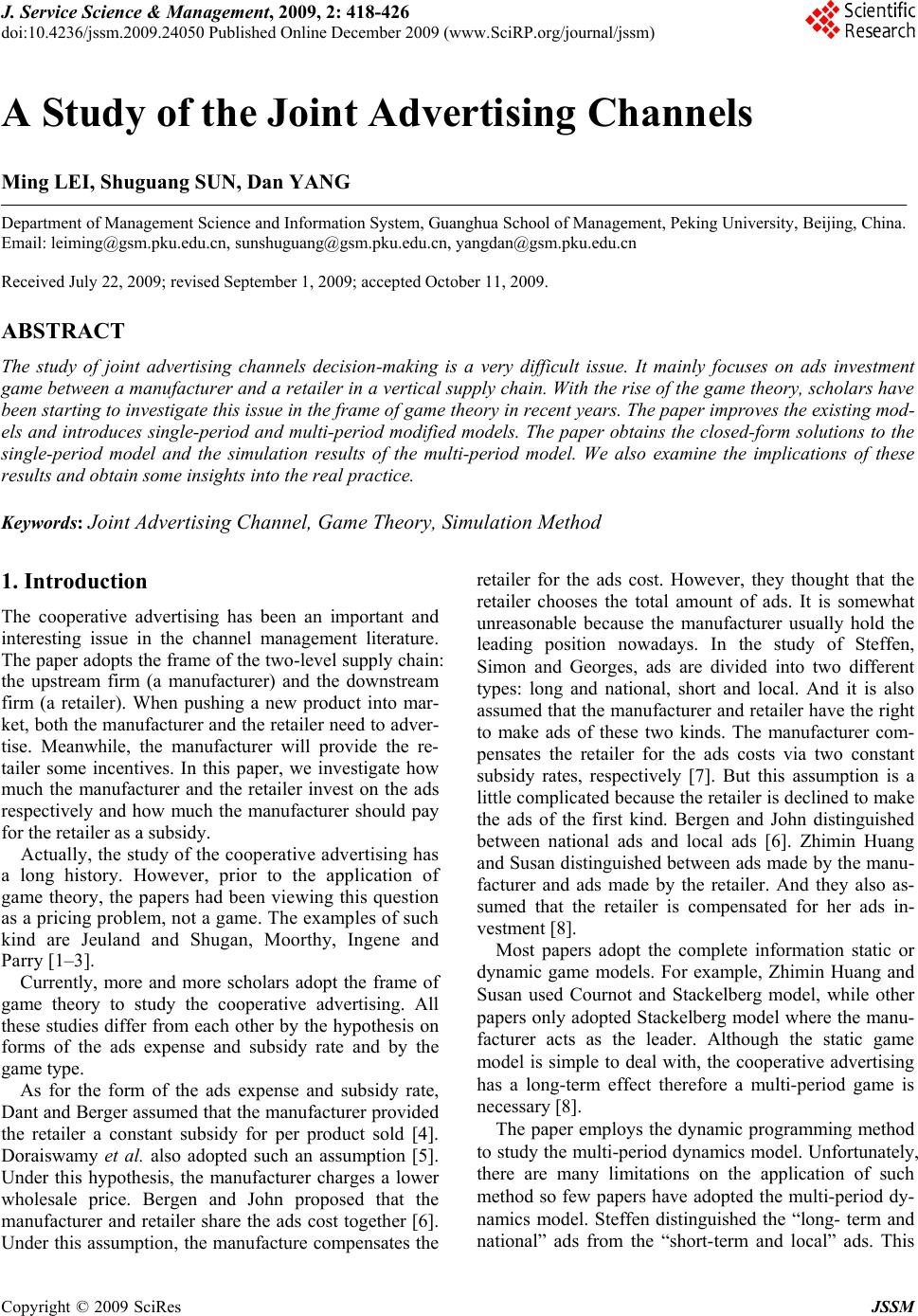J. Service Science & Management, 2009, 2: 418-426
doi:10.4236/jssm.2009.24050 Published Online December 2009 (www.SciRP.org/journal/jssm)
A Study of the Joint Advertising Channels
Ming LEI, Shuguang SUN, Dan YANG
Department of Management Science and Information System, Guanghua School of Management, Peking University, Beijing, China.
Received July 22, 2009; revised September 1, 2009; accepted October 11, 2009.
ABSTRACT
The study of joint advertising channels decision-making is a very difficult issue. It mainly focuses on ads investment
game between a manufacturer and a retailer in a vertical supply chain. With the rise of the game theory, scholars have
been starting to investigate this issue in the frame of game theory in recent years. The paper improves the existing mod-
els and introduces single-period and multi-period modified models. The paper obtains the closed-form solutions to the
single-period model and the simulation results of the multi-period model. We also examine the implications of these
results and obtain some insights into the real practice.
Keywords: Joint Advertising Channel, Game Theory, Simulation Method
1. Introduction
The cooperative advertising has been an important and
interesting issue in the channel management literature.
The paper adopts the frame of the two-level supply chain:
the upstream firm (a manufacturer) and the downstream
firm (a retailer). When pushing a new product into mar-
ket, both the manufacturer and the retailer need to adver-
tise. Meanwhile, the manufacturer will provide the re-
tailer some incentives. In this paper, we investigate how
much the manufacturer and the retailer invest on the ads
respectively and how much the manufacturer should pay
for the retailer as a subsidy.
Actually, the study of the cooperative advertising has
a long history. However, prior to the application of
game theory, the papers had been viewing this question
as a pricing problem, not a game. The examples of such
kind are Jeuland and Shugan, Moorthy, Ingene and
Parry [1–3].
Currently, more and more scholars adopt the frame of
game theory to study the cooperative advertising. All
these studies differ from each other by the hypothesis on
forms of the ads expense and subsidy rate and by the
game type.
As for the form of the ads expense and subsidy rate,
Dant and Berger assumed that the manufacturer provided
the retailer a constant subsidy for per product sold [4].
Doraiswamy et al. also adopted such an assumption [5].
Under this hypothesis, the manufacturer charges a lower
wholesale price. Bergen and John proposed that the
manufacturer and retailer share the ads cost together [6].
Under this assumption, the manufacture compensates the
retailer for the ads cost. However, they thought that the
retailer chooses the total amount of ads. It is somewhat
unreasonable because the manufacturer usually hold the
leading position nowadays. In the study of Steffen,
Simon and Georges, ads are divided into two different
types: long and national, short and local. And it is also
assumed that the manufacturer and retailer have the right
to make ads of these two kinds. The manufacturer com-
pensates the retailer for the ads costs via two constant
subsidy rates, respectively [7]. But this assumption is a
little complicated because the retailer is declined to make
the ads of the first kind. Bergen and John distinguished
between national ads and local ads [6]. Zhimin Huang
and Susan distinguished between ads made by the manu-
facturer and ads made by the retailer. And they also as-
sumed that the retailer is compensated for her ads in-
vestment [8].
Most papers adopt the complete information static or
dynamic game models. For example, Zhimin Huang and
Susan used Cournot and Stackelberg model, while other
papers only adopted Stackelberg model where the manu-
facturer acts as the leader. Although the static game
model is simple to deal with, the cooperative advertising
has a long-term effect therefore a multi-period game is
necessary [8].
The paper employs the dynamic programming method
to study the multi-period dynamics model. Unfortunately,
there are many limitations on the application of such
method so few papers have adopted the multi-period dy-
namics model. Steffen distinguished the “long- term and
national” ads from the “short-term and local” ads. This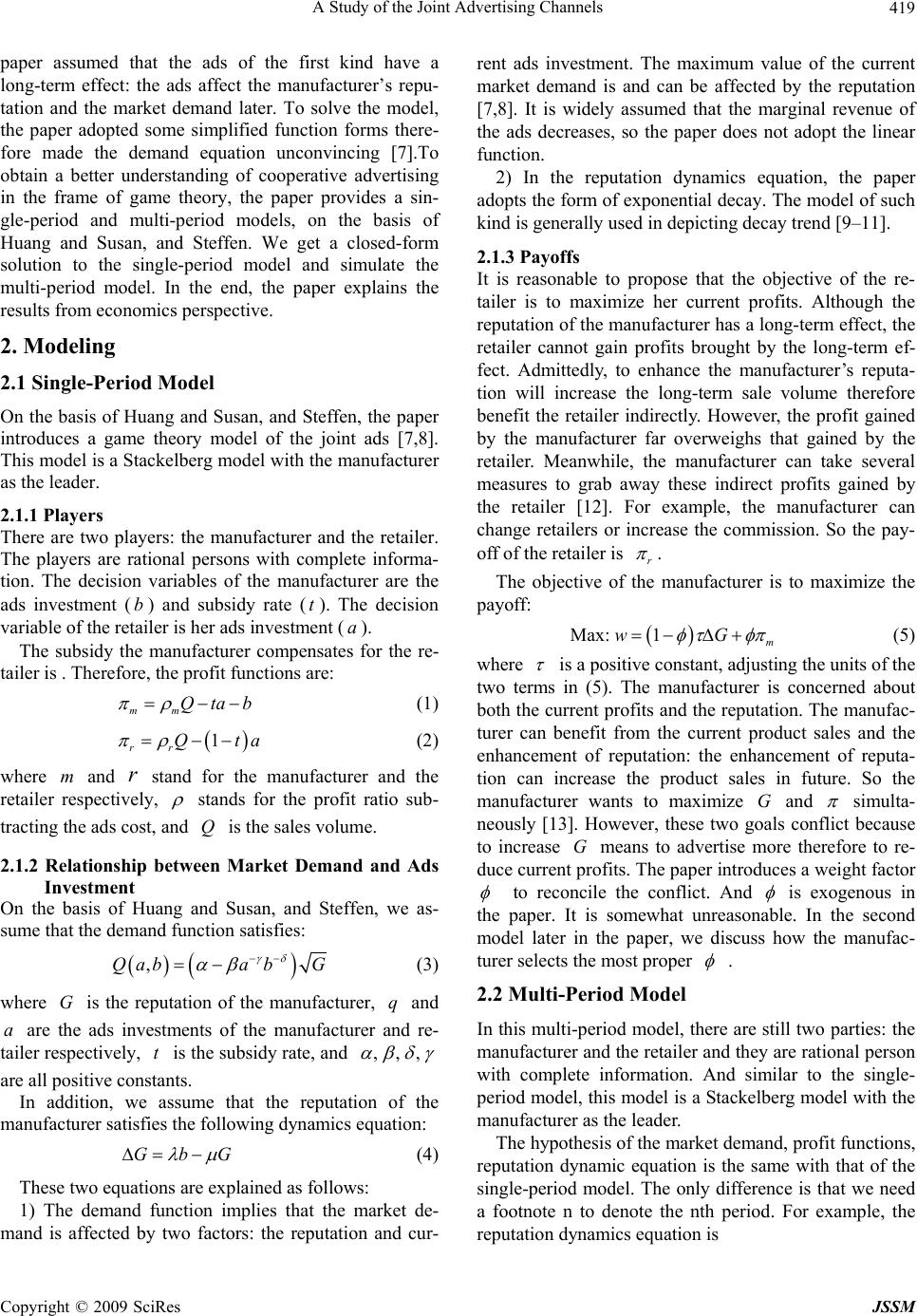

A Study of the Joint Advertising Channels419
paper assumed that the ads of the first kind have a
long-term effect: the ads affect the manufacturer’s repu-
tation and the market demand later. To solve the model,
the paper adopted some simplified function forms there-
fore made the demand equation unconvincing [7].To
obtain a better understanding of cooperative advertising
in the frame of game theory, the paper provides a sin-
gle-period and multi-period models, on the basis of
Huang and Susan, and Steffen. We get a closed-form
solution to the single-period model and simulate the
multi-period model. In the end, the paper explains the
results from economics perspective.
2. Modeling
2.1 Single-Period Model
On the basis of Huang and Susan, and Steffen, the paper
introduces a game theory model of the joint ads [7,8].
This model is a Stackelberg model with the manufacturer
as the leader.
2.1.1 Players
There are two players: the manufacturer and the retailer.
The players are rational persons with complete informa-
tion. The decision variables of the manufacturer are the
ads investment () and subsidy rate (). The decision
variable of the retailer is her ads investment ().
bt
a
The subsidy the manufacturer compensates for the re-
tailer is . Therefore, the profit functions are:
mm
Qtab

  (1)

1
rr
Qt  a (2)
where and stand for the manufacturer and the
retailer respectively,
mr

stands for the profit ratio sub-
tracting the ads cost, and is the sales volume. Q
2.1.2 Relationship between Market Demand and Ads
Investment
On the basis of Huang and Susan, and Steffen, we as-
sume that the demand function satisfies:
 
,Qaba bG



 (3)
where is the reputation of the manufacturer, and
are the ads investments of the manufacturer and re-
tailer respectively, is the subsidy rate, and
G q
,,
a
t,


are all positive constants.
In addition, we assume that the reputation of the
manufacturer satisfies the following dynamics equation:
GbG

   (4)
These two equations are explained as follows:
1) The demand function implies that the market de-
mand is affected by two factors: the reputation and cur-
rent ads investment. The maximum value of the current
market demand is and can be affected by the reputation
[7,8]. It is widely assumed that the marginal revenue of
the ads decreases, so the paper does not adopt the linear
function.
2) In the reputation dynamics equation, the paper
adopts the form of exponential decay. The model of such
kind is generally used in depicting decay trend [9–11].
2.1.3 Payoffs
It is reasonable to propose that the objective of the re-
tailer is to maximize her current profits. Although the
reputation of the manufacturer has a long-term effect, the
retailer cannot gain profits brought by the long-term ef-
fect. Admittedly, to enhance the manufacturer’s reputa-
tion will increase the long-term sale volume therefore
benefit the retailer indirectly. However, the profit gained
by the manufacturer far overweighs that gained by the
retailer. Meanwhile, the manufacturer can take several
measures to grab away these indirect profits gained by
the retailer [12]. For example, the manufacturer can
change retailers or increase the commission. So the pay-
off of the retailer is r

.
The objective of the manufacturer is to maximize the
payoff:


Max: 1m wG

   (5)
where

is a positive constant, adjusting the units of the
two terms in (5). The manufacturer is concerned about
both the current profits and the reputation. The manufac-
turer can benefit from the current product sales and the
enhancement of reputation: the enhancement of reputa-
tion can increase the product sales in future. So the
manufacturer wants to maximize and G

simulta-
neously [13]. However, these two goals conflict because
to increase means to advertise more therefore to re-
duce current profits. The paper introduces a weight factor
G

to reconcile the conflict. And

is exogenous in
the paper. It is somewhat unreasonable. In the second
model later in the paper, we discuss how the manufac-
turer selects the most proper

.
2.2 Multi-Period Model
In this multi-period model, there are still two parties: the
manufacturer and the retailer and they are rational person
with complete information. And similar to the single-
period model, this model is a Stackelberg model with the
manufacturer as the leader.
The hypothesis of the market demand, profit functions,
reputation dynamic equation is the same with that of the
single-period model. The only difference is that we need
a footnote n to denote the nth period. For example, the
reputation dynamics equation is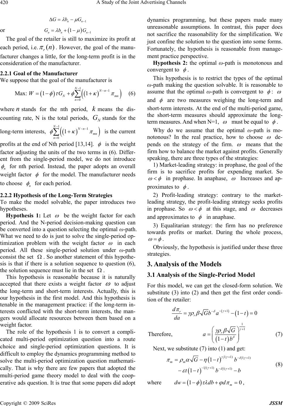

A Study of the Joint Advertising Channels 420
1nn
Gb G



 
or


1
1
nn n
Gb G 


The goal of the retailer is still to maximize its profit at
each period, i.e.()
rn

. However, the goal of the manu-
facturer changes a little, for the long-term profit is in the
consideration of the manufacturer.
2.2.1 Goal of the Manufacturer
We suppose that the goal of the manufacturer is
 

11
0
Max: 11
NNn
Nm
n
WG  


 
  n

(6)
where stands for the nth period, kmeans the dis-
counting rate, N is the total periods, stands for the
long-term interests, is the current
profits at the end of Nth period [13,14].
n
N

G
mn


11
0
1
NNn
n






is the weight
factor adjusting the units of the two terms in (6). Differ-
ent from the single-period model, we do not introduce
n

for nth period. Instead, the paper adopts an overall
weight factor

for the model. The manufacturer needs
to choose n

for each period.
2.2.2 Hypothesis of the Long-Term Strategies
To make the model solvable, the paper introduces two
hypotheses.
Hypothesis 1: Let

be the weight factor for each
period. And the N-period decision-making question can
be converted into a question selecting the optimal ω-path.
What we need to do is just to solve the single-period op-
timization problem with the weight factor

in each
period. All these single-period solution under ω-path
consist the set . So another statement of this hypothe-
sis is that if there is a solution sequence to question (6),
the solution sequence must lie in the set .


This hypothesis is reasonable because it is naturally
accepted that there exists a weight factor

to adjust
the long-term and short-term interests. Actually, this is
our hypothesis in the first model. And this hypothesis is
tenable in the management practice: if the long-term in-
terests conflicted with the short-term interests, the man-
gers would allocate resources between them based on a
weight factor.
The role of the hypothesis 1 is to convert a compli-
cated multi-period optimization question into a route
choice and single-period optimization questions. It is
difficult to employ the dynamics programming method to
solve the multi-period optimization question mathemati-
cally. That is why there are few papers that adopted the
multi-period game theory model to deal with the coop-
erative ads question. It is true that some papers did adopt
dynamics programming, but these papers made many
unreasonable assumptions. In contrast, this paper does
not sacrifice the reasonability for the simplification. We
just confine the solution to the question into some forms.
Fortunately, the hypothesis is reasonable from manage-
ment practice perspective.
Hypothesis 2: the optimal ω-path is monotonous and
convergent to

.
This hypothesis is to restrict the types of the optimal
ω-path making the question solvable. It is reasonable to
assume that the optimal ω-path is convergent to

:

and

are two measures weighing the long-term and
short-term interests. At the end of the multi-period game,
the short-term measures should approximate the long-
term measures. And when N=1,

must be equal to

.
Why do we assume that the optimal ω-path is mo-
notonous? In the real practice, how to choose

de-
pends on the strategy of the firm.

means that the
firm how to balance the market against profits. Generally
speaking, there are three types of the strategies:
1) Market-leading strategy: in prophase, the goal of the
firm is to sacrifice profits for expending market. So



in prophase. In anaphase,

Increases and ap-
proximates to

.
2) Profit-leading strategy: contrary to the market-
leading strategy, the profit-leading strategy seeks profits
in prophase. So



at this stage, and

decreases
and approximates to

in anaphase.
3) Equalitarian strategy: the firm has no preference
towards profits or market. During the whole process,



.
Obviously, the hypothesis is justified under these three
strategies.
3. Analysis of the Models
3.1 Analysis of the Single-Period Model
For this model, we can get the closed-form solution. We
substitute (3) into (2) and then get the first order condi-
tion of the retailer:


110
r
r
dGb at
da


 




Therefore,

1
1
1
rG
atb


 








(7)
Next, we substitute (7) into (1) and get:


(1) (1)
1( 1)(1)
1
1
mm
Gtb
tt bb
 

 


 

 (8)
where


10
m
dwdb d  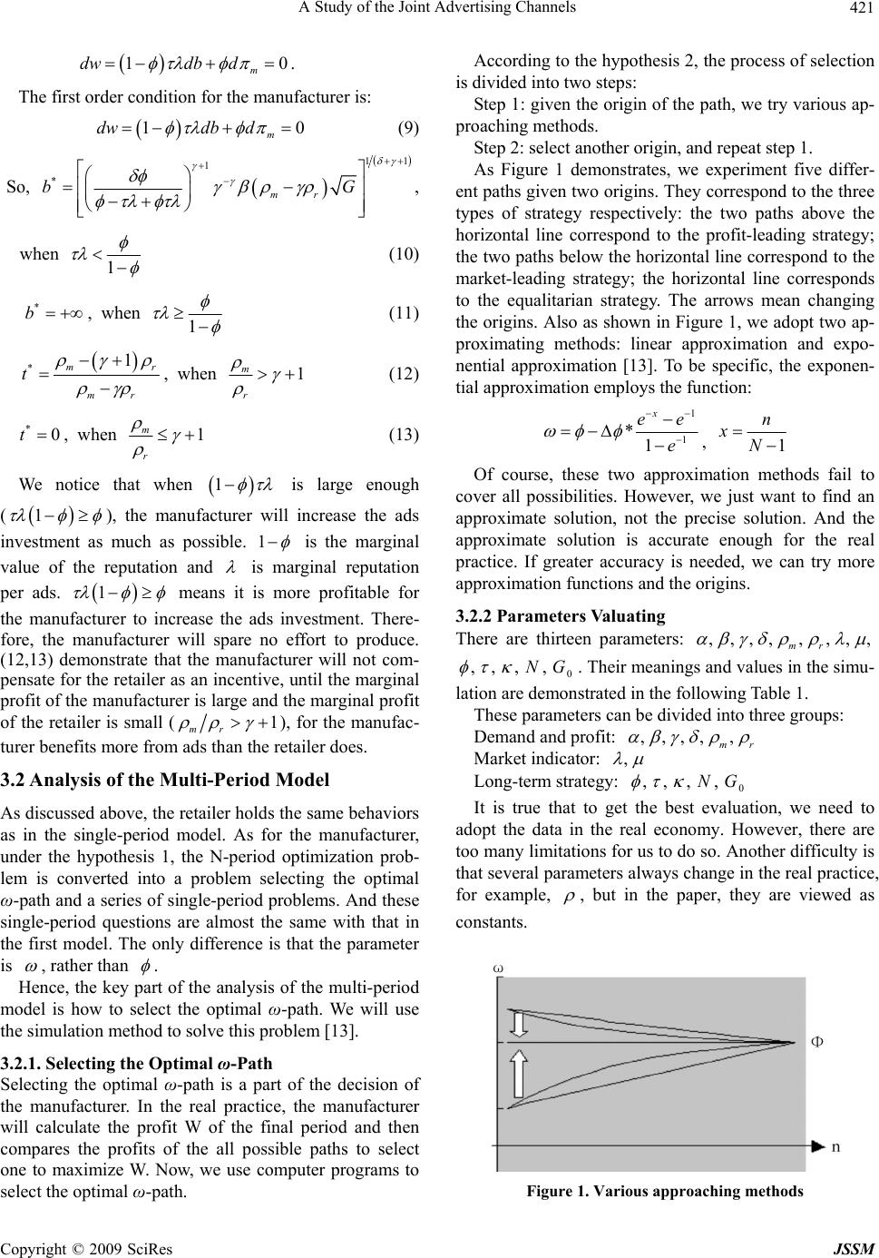

,

A Study of the Joint Advertising Channels421

10
m
dwdb d    .
The first order condition for the manufacturer is:

10
m
dwdb d     (9)
So,



11
1
*
mr
b



  

G






 


 





,
when 1



 (10)
, when 1



 (11)
*
b

*1
mr
mr
t



, when 1
m
r



 (12)
, when 1
m
r


 (13)
*0t
We notice that when

1

  is large enough
(

1

   ), the manufacturer will increase the ads
investment as much as possible. 1

 is the marginal
value of the reputation and

is marginal reputation
per ads.

1

   means it is more profitable for
the manufacturer to increase the ads investment. There-
fore, the manufacturer will spare no effort to produce.
(12,13) demonstrate that the manufacturer will not com-
pensate for the retailer as an incentive, until the marginal
profit of the manufacturer is large and the marginal profit
of the retailer is small (1
mr

 ), for the manufac-
turer benefits more from ads than the retailer does.
3.2 Analysis of the Multi-Period Model
As discussed above, the retailer holds the same behaviors
as in the single-period model. As for the manufacturer,
under the hypothesis 1, the N-period optimization prob-
lem is converted into a problem selecting the optimal
ω-path and a series of single-period problems. And these
single-period questions are almost the same with that in
the first model. The only difference is that the parameter
is

, rather than

.
Hence, the key part of the analysis of the multi-period
model is how to select the optimal ω-path. We will use
the simulation method to solve this problem [13].
3.2.1. Selecti ng the Optimal ω-Path
Selecting the optimal ω-path is a part of the decision of
the manufacturer. In the real practice, the manufacturer
will calculate the profit W of the final period and then
compares the profits of the all possible paths to select
one to maximize W. Now, we use computer programs to
select the optimal ω-path.
According to the hypothesis 2, the process of selection
is divided into two steps:
Step 1: given the origin of the path, we try various ap-
proaching methods.
Step 2: select another origin, and repeat step 1.
As Figure 1 demonstrates, we experiment five differ-
ent paths given two origins. They correspond to the three
types of strategy respectively: the two paths above the
horizontal line correspond to the profit-leading strategy;
the two paths below the horizontal line correspond to the
market-leading strategy; the horizontal line corresponds
to the equalitarian strategy. The arrows mean changing
the origins. Also as shown in Figure 1, we adopt two ap-
proximating methods: linear approximation and expo-
nential approximation [13]. To be specific, the exponen-
tial approximation employs the function:
1
1
*1
x
ee
e
 




, 1
n
xN 
Of course, these two approximation methods fail to
cover all possibilities. However, we just want to find an
approximate solution, not the precise solution. And the
approximate solution is accurate enough for the real
practice. If greater accuracy is needed, we can try more
approximation functions and the origins.
3.2.2 Parameters Valuating
There are thirteen parameters: ,,,,, ,,,
mr

 
0
,, ,,NG

 . Their meanings and values in the simu-
lation are demonstrated in the following Table 1.
These parameters can be divided into three groups:
Demand and profit: ,,,, ,
mr

 
, Market indicator:


Long-term strategy: 0 ,, ,,NG


It is true that to get the best evaluation, we need to
adopt the data in the real economy. However, there are
too many limitations for us to do so. Another difficulty is
that several parameters always change in the real practice,
for example,

, but in the paper, they are viewed as
constants.
Figure 1. Various approaching methods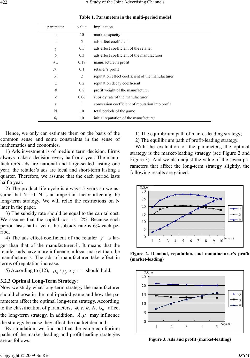

A Study of the Joint Advertising Channels 422
Table 1. Parameters in the multi-period model
parameter value implication
α 10 market capacity
β 5 ads effect coefficient
γ 0.5 ads effect coefficient of the retailer
δ 0.3 ads effect coefficient of the manufacturer
m

0.18 manufacturer’s profit
r

0.1 retailer’s profit

2 reputation effect coefficient of the manufacturer
μ 0.2 reputation decay coefficient

0.8 profit weight of the manufacturer
κ 0.06 subsidy rate of the manufacturer
τ 1 conversion coefficient of reputation into profit
N 10 total periods of the game
0
G 10 initial reputation of the manufacturer
Hence, we only can estimate them on the basis of the
common sense and some constraints in the sense of
mathematics and economics.
1) The equilibrium path of market-leading strategy;
2) The equilibrium path of profit-leading strategy.
With the evaluation of the parameters, the optimal
strategy is the market-leading strategy (see Figure 2 and
Figure 3). And we also adjust the value of the seven pa-
rameters that affect the long-term strategy slightly, the
following results are gained:
1) Ads investment is of medium term decision. Firms
always make a decision every half or a year. The manu-
facturer’s ads are national and large-scaled lasting one
year; the retailer’s ads are local and short-term lasting a
quarter. Therefore, we assume that the each period lasts
half a year.
2) The product life cycle is always 5 years so we as-
sume that N=10. N is an important factor affecting the
long-term strategy. We will relax the restrictions on N
later in the paper.
3) The subsidy rate should be equal to the capital cost.
We assume that the capital cost is 12%. Because each
period lasts half a year, the subsidy rate is 6% each pe-
riod.
4) The ads effect coefficient of the retailer

is lar-
ger than that of the manufactuerr

. It means that the
retailer’ ads have more influence in local market than the
manufacturer’s. The ads of manufacturer take effect in
terms of reputation increase.
Figure 2. Demand, reputation, and manufacturer’s profit
(market-leading)
5) According to (12), /
mr 1

 
should hold.
3.2.3 Optimal Long-Term Strategy:
Now we study what long-term strategy the manufacturer
should choose in the multi-period game and how the pa-
rameters affect the optimal long-term strategy. According
to the classification of parameters, 0 ,, ,,NG


, affect the long-term strategy. In addition,


may influence
the strategy because they affect the market demand.
By simulation, we find out that the game equilibrium
paths of the market-leading and profit-leading strategies
are as follows: Figure 3. Ads and profit (market-leading)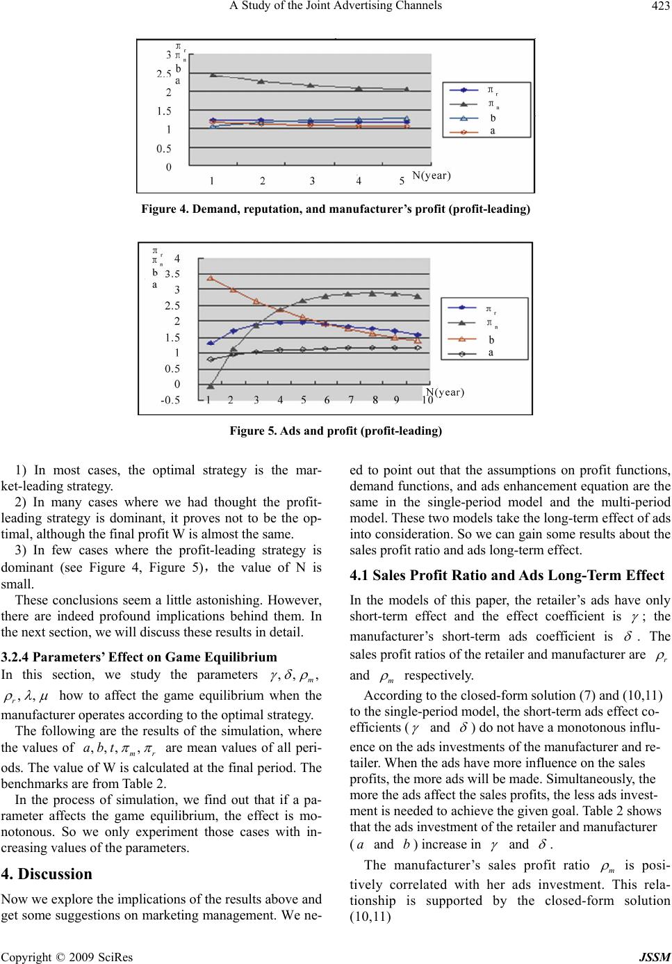

A Study of the Joint Advertising Channels423
Figure 4. Demand, reputation, and manufacturer’s profit (profit-leading)
Figure 5. Ads and profit (profit-leading)
1) In most cases, the optimal strategy is the mar-
ket-leading strategy.
2) In many cases where we had thought the profit-
leading strategy is dominant, it proves not to be the op-
timal, although the final profit W is almost the same.
3) In few cases where the profit-leading strategy is
dominant (see Figure 4, Figure 5)，the value of N is
small.
These conclusions seem a little astonishing. However,
there are indeed profound implications behind them. In
the next section, we will discuss these results in detail.
3.2.4 Parameters’ Effect on Game Equilibrium
In this section, we study the parameters ,, ,
m


,,
r


how to affect the game equilibrium when the
manufacturer operates according to the optimal strategy.
The following are the results of the simulation, where
the values of ,,, ,
mr
abt

 are mean values of all peri-
ods. The value of W is calculated at the final period. The
benchmarks are from Table 2.
In the process of simulation, we find out that if a pa-
rameter affects the game equilibrium, the effect is mo-
notonous. So we only experiment those cases with in-
creasing values of the parameters.
4. Discussion
Now we explore the implications of the results above and
get some suggestions on marketing management. We ne-
ed to point out that the assumptions on profit functions,
demand functions, and ads enhancement equation are the
same in the single-period model and the multi-period
model. These two models take the long-term effect of ads
into consideration. So we can gain some results about the
sales profit ratio and ads long-term effect.
4.1 Sales Profit Ratio and Ads Long-Term Effect
In the models of this paper, the retailer’s ads have only
short-term effect and the effect coefficient is

; the
manufacturer’s short-term ads coefficient is

. The
sales profit ratios of the retailer and manufacturer are r

and m

respectively.
According to the closed-form solution (7) and (10,11)
to the single-period model, the short-term ads effect co-
efficients (

and

) do not have a monotonous influ-
ence on the ads investments of the manufacturer and re-
tailer. When the ads have more influence on the sales
profits, the more ads will be made. Simultaneously, the
more the ads affect the sales profits, the less ads invest-
ment is needed to achieve the given goal. Table 2 shows
that the ads investment of the retailer and manufacturer
(a and ) increase in b

and

.
The manufacturer’s sales profit ratio m

is posi-
tively correlated with her ads investment. This rela-
tionship is supported by the closed-form solution
(10,11)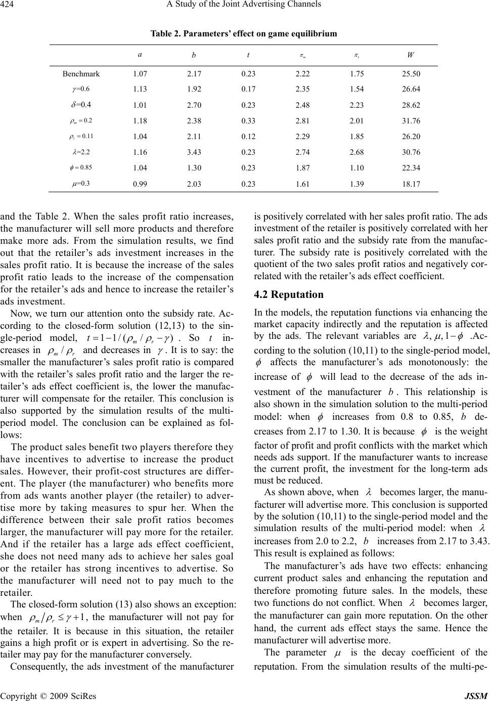

A Study of the Joint Advertising Channels 424
Table 2. Parameters’ effect on game equilibrium
a b t m

r

W
Benchmark 1.07 2.17 0.23 2.22 1.75 25.50
=0.6

1.13 1.92 0.17 2.35 1.54 26.64
=0.4

1.01 2.70 0.23 2.48 2.23 28.62
0.2
m
  1.18 2.38 0.33 2.81 2.01 31.76
0.11
r
  1.04 2.11 0.12 2.29 1.85 26.20
=2.2

1.16 3.43 0.23 2.74 2.68 30.76
0.85

 1.04 1.30 0.23 1.87 1.10 22.34
=0.3

0.99 2.03 0.23 1.61 1.39 18.17
and the Table 2. When the sales profit ratio increases,
the manufacturer will sell more products and therefore
make more ads. From the simulation results, we find
out that the retailer’s ads investment increases in the
sales profit ratio. It is because the increase of the sales
profit ratio leads to the increase of the compensation
for the retailer’s ads and hence to increase the retailer’s
ads investment.
Now, we turn our attention onto the subsidy rate. Ac-
cording to the closed-form solution (12,13) to the sin-
gle-period model, 11/( /)
mr
t

  . So in-
creases in r
t
/
m


and decreases in

. It is to say: the
smaller the manufacturer’s sales profit ratio is compared
with the retailer’s sales profit ratio and the larger the re-
tailer’s ads effect coefficient is, the lower the manufac-
turer will compensate for the retailer. This conclusion is
also supported by the simulation results of the multi-
period model. The conclusion can be explained as fol-
lows:
The product sales benefit two players therefore they
have incentives to advertise to increase the product
sales. However, their profit-cost structures are differ-
ent. The player (the manufacturer) who benefits more
from ads wants another player (the retailer) to adver-
tise more by taking measures to spur her. When the
difference between their sale profit ratios becomes
larger, the manufacturer will pay more for the retailer.
And if the retailer has a large ads effect coefficient,
she does not need many ads to achieve her sales goal
or the retailer has strong incentives to advertise. So
the manufacturer will need not to pay much to the
retailer.
The closed-form solution (13) also shows an exception:
when 1
mr

 , the manufacturer will not pay for
the retailer. It is because in this situation, the retailer
gains a high profit or is expert in advertising. So the re-
tailer may pay for the manufacturer conversely.
Consequently, the ads investment of the manufacturer
is positively correlated with her sales profit ratio. The ads
investment of the retailer is positively correlated with her
sales profit ratio and the subsidy rate from the manufac-
turer. The subsidy rate is positively correlated with the
quotient of the two sales profit ratios and negatively cor-
related with the retailer’s ads effect coefficient.
4.2 Reputation
In the models, the reputation functions via enhancing the
market capacity indirectly and the reputation is affected
by the ads. The relevant variables are ,,1



.Ac-
cording to the solution (10,11) to the single-period model,

affects the manufacturer’s ads monotonously: the
increase of

will lead to the decrease of the ads in-
vestment of the manufacturer b. This relationship is
also shown in the simulation solution to the multi-period
model: when

increases from 0.8 to 0.85, de-
creases from 2.17 to 1.30. It is because
b

is the weight
factor of profit and profit conflicts with the market which
needs ads support. If the manufacturer wants to increase
the current profit, the investment for the long-term ads
must be reduced.
As shown above, when

becomes larger, the manu-
facturer will advertise more. This conclusion is supported
by the solution (10,11) to the single-period model and the
simulation results of the multi-period model: when

increases from 2.0 to 2.2, increases from 2.17 to 3.43.
This result is explained as follows:
b
The manufacturer’s ads have two effects: enhancing
current product sales and enhancing the reputation and
therefore promoting future sales. In the models, these
two functions do not conflict. When

becomes larger,
the manufacturer can gain more reputation. On the other
hand, the current ads effect stays the same. Hence the
manufacturer will advertise more.
The parameter

is the decay coefficient of the
reputation. From the simulation results of the multi-pe-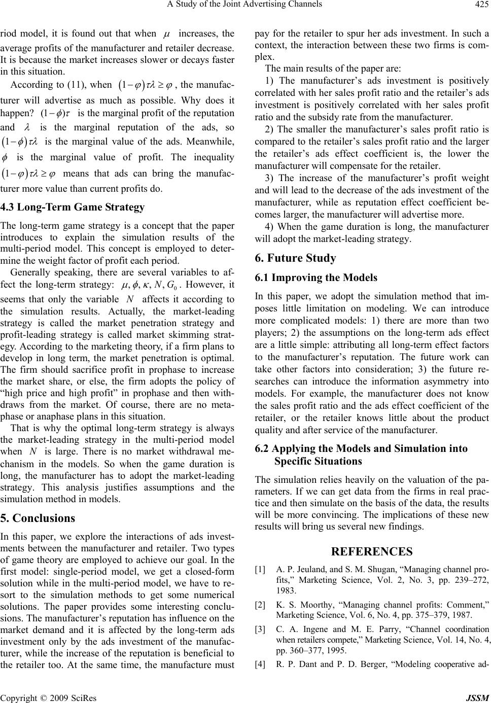

A Study of the Joint Advertising Channels425
riod model, it is found out that when

increases, the
average profits of the manufacturer and retailer decrease.
It is because the market increases slower or decays faster
in this situation.
According to (11), when

1

 

, the manufac-
turer will advertise as much as possible. Why does it
happen? (1 )

  is the marginal profit of the reputation
and

is the marginal reputation of the ads, so

1


  is the marginal value of the ads. Meanwhile,

is the marginal value of profit. The inequality

1

    means that ads can bring the manufac-
turer more value than current profits do.
4.3 Long-Term Game Strategy
The long-term game strategy is a concept that the paper
introduces to explain the simulation results of the
multi-period model. This concept is employed to deter-
mine the weight factor of profit each period.
Generally speaking, there are several variables to af-
fect the long-term strategy: 0 ,NG,,,


N
. However, it
seems that only the variable affects it according to
the simulation results. Actually, the market-leading
strategy is called the market penetration strategy and
profit-leading strategy is called market skimming strat-
egy. According to the marketing theory, if a firm plans to
develop in long term, the market penetration is optimal.
The firm should sacrifice profit in prophase to increase
the market share, or else, the firm adopts the policy of
“high price and high profit” in prophase and then with-
draws from the market. Of course, there are no meta-
phase or anaphase plans in this situation.
That is why the optimal long-term strategy is always
the market-leading strategy in the multi-period model
when is large. There is no market withdrawal me-
chanism in the models. So when the game duration is
long, the manufacturer has to adopt the market-leading
strategy. This analysis justifies assumptions and the
simulation method in models.
N
5. Conclusions
In this paper, we explore the interactions of ads invest-
ments between the manufacturer and retailer. Two types
of game theory are employed to achieve our goal. In the
first model: single-period model, we get a closed-form
solution while in the multi-period model, we have to re-
sort to the simulation methods to get some numerical
solutions. The paper provides some interesting conclu-
sions. The manufacturer’s reputation has influence on the
market demand and it is affected by the long-term ads
investment only by the ads investment of the manufac-
turer, while the increase of the reputation is beneficial to
the retailer too. At the same time, the manufacture must
pay for the retailer to spur her ads investment. In such a
context, the interaction between these two firms is com-
plex.
The main results of the paper are:
1) The manufacturer’s ads investment is positively
correlated with her sales profit ratio and the retailer’s ads
investment is positively correlated with her sales profit
ratio and the subsidy rate from the manufacturer.
2) The smaller the manufacturer’s sales profit ratio is
compared to the retailer’s sales profit ratio and the larger
the retailer’s ads effect coefficient is, the lower the
manufacturer will compensate for the retailer.
3) The increase of the manufacturer’s profit weight
and will lead to the decrease of the ads investment of the
manufacturer, while as reputation effect coefficient be-
comes larger, the manufacturer will advertise more.
4) When the game duration is long, the manufacturer
will adopt the market-leading strategy.
6. Future Study
6.1 Improving the Models
In this paper, we adopt the simulation method that im-
poses little limitation on modeling. We can introduce
more complicated models: 1) there are more than two
players; 2) the assumptions on the long-term ads effect
are a little simple: attributing all long-term effect factors
to the manufacturer’s reputation. The future work can
take other factors into consideration; 3) the future re-
searches can introduce the information asymmetry into
models. For example, the manufacturer does not know
the sales profit ratio and the ads effect coefficient of the
retailer, or the retailer knows little about the product
quality and after service of the manufacturer.
6.2 Applying the Models and Simulation into
Specific Situations
The simulation relies heavily on the valuation of the pa-
rameters. If we can get data from the firms in real prac-
tice and then simulate on the basis of the data, the results
will be more convincing. The implications of these new
results will bring us several new findings.
REFERENCES
[1] A. P. Jeuland, and S. M. Shugan, “Managing channel pro-
fits,” Marketing Science, Vol. 2, No. 3, pp. 239–272,
1983.
[2] K. S. Moorthy, “Managing channel profits: Comment,”
Marketing Science, Vol. 6, No. 4, pp. 375–379, 1987.
[3] C. A. Ingene and M. E. Parry, “Channel coordination
when retailers compete,” Marketing Science, Vol. 14, No. 4,
pp. 360–377, 1995.
[4] R. P. Dant and P. D. Berger, “Modeling cooperative ad-

A Study of the Joint Advertising Channels 426
vertising decisions in franchising,” Journal of the Opera-
tional Research Society, Vol. 49, No. 9, pp. 1120–1136,
1996.
[5] K. Doraiswamy, T. W. McGuire, and R. Staelin, “An
analysis of alternative advertising strategies in a competi-
tive franchise framework,” Proceedings of Educator's
Conference of American Marketing Association, pp. 463–
467, 1979.
[6] M. Bergen and G. John, “Understanding cooperative ad-
vertising participation rates in conventional channels,”
Journal of Marketing Research, Vol. 34, No. 3, pp. 357–
369, 1997.
[7] S. Jørgensen, S. P. Sigue, and G. Zaccour, “Dynamic
cooperative advertising in a channel,” Journal of Retailing,
Vol. 76, No. 1, pp. 71–91, 2000.
[8] Z. Huang and S. X. Li, “Co-op advertising models in
manufacturer-retailer supply chains: A game theory ap-
proach,” European Journal of Operational Research, Vol.
135, No. 3, pp. 527–544, 2001.
[9] Deal and R. Kenneth, “Optimizing advertising expendi-
tures in a dynamic duopoly,” Operations Research, Vol.
27, No. 4, pp. 682–692, 1979.
[10] Chintagunta, K. Pradeep and D. Jain, “A dynamic model
of channel member strategies for marketing expenditures,”
Marketing Science, Vol. 11, No. 2, pp. 168–188, 1992.
[11] Chintagunta and K. Pradeep, “Investigating the sensitivity
of equilibrium profits to advertising dynamics and com-
petitive effects”, Management Science, Vol. 39, No. 9, pp.
1146–1162, 1993.
[12] K. C. Sen, “Advertising fees in the franchised channel,”
Journal of Marketing Channels, Vol. 4, No. 1, pp. 83–101,
1995.
[13] S. P. Wang, K. L. Judd and C. Gung, “Solving a savings
allocation problem by numerical dynamic programming
with shape-preserving interpolation,” Computers & Op-
erations Research, Vol. 27, pp. 399–408, 2000.
[14] L. Tesfatsion, “Introduction to the special issue on agent-
based computational economics,” Journal of Economic
Dynamics and Control, Vol. 25, No. 3–4, pp. 281–293,
2001.