J. Service Science & Management, 2009, 2: 368-377
doi:10.4236/jssm.2009.24044 Published Online December 2009 (www.SciRP.org/journal/jssm)
Revenue and Duration of Oral Auction
Junmin SHI, Ai-Chih CHANG
Department of Supply Chain Management & Marketing Sciences, Rutgers University, Newark, USA.
Received July 13, 2009; revised August 22, 2009; accepted October 5, 2009.
ABSTRACT
This paper in vestigates the revenue and duratio n of a well-known h ybrid oral auction (English auction and Dutch auc-
tion) that is extensively adopted in practice, for instance the Christie’s. Unlike sealed bid auction, oral auction is fea-
tured by its complexity of dynamic process. The bidding price varies as a stochastic time series. Therefore, the duration
of oral auction as well as its revenue performs randomly. From the seller’s perspective, both the revenue and the dura-
tion are so important that extra attention and effort should be put on auction design. One of the most important issues is
how to choose the starting bid price to maximize its revenue or minimize its duration. In this paper, the bidding process
is decomposed into two phases: English auction (descending-bid) phase and the Dutch auction (ascending-bid) phase.
For each phase, with the aid of Markov method, we derive the expected revenue and duration as a function of the start-
ing bid. For an oral auction with a large number of bidder and each bidder behaves independently, we provide the limit
results of the expected revenue and duration. The results of the auction model can be easily implemented in auction
design.
Keywords: Duration, Dutch Auction, English Auction, Oral Auction, Revenue
1. Introduction
As a powerful and well-known tool in business markets,
auction plays an important role in selling objects espe-
cially for antiques and art. With a long history around the
world, auctions are very common for the commodities su ch
as tobacco, fish, cattle, racehorses, and anything that has
a market of multiple people interested in purchasing. Th e
main reason why auction is so common is that a group of
people are interested in buying the same object, and t her eb y
offering their individual bids on the object. Serving as a
tool that takes all the interested buyers into one game,
auction decides the winner (usually the highest bidder) of
the game.
Recently, the auction theory has been well developed
systematically in practice and academy as well. Generally
speaking , there are four typ es of auction that are used for
the alloca tion of a single item: Th ese four standard au cti o n s
are the English auction, the Dutch auction, the First-Price
Sealed-Bid auction, and the Second-Price Sealed-Bid auc-
tion. The context for each type of auction is explained briefl y
as follows. We refer the interested reader to [1].
 Open ascending-bid auctions (English auctions) is
commonly referred to as oral outcry auctions, in which
the price is steadily raised by the auctioneer with bidders
dropping out once the price becomes too high. This con-
tinues until there remains only one bidder (the highest
bidder) who wins the auction at the current price.
 Open descending-bid auctions (Dutch auctions) in
which the price starts at a level sufficiently high to deter
all bidders and is progressively lowered until a bidder
indicates to buy at the current price. The bidder wins the
auction and pays the price at which he or she bid.
 First-price sealed-bid auctions in which bidders
place their bid in a sealed envelope and simultaneously
hand them in to the auctioneer. The envelopes are opened
and the bidder with the highest bid wins, paying a price at
which he or sh e bid .
 Second-price sealed-bid auctions (Vickrey auctions)
in which bidders place their bid in a sealed envelope and
simultaneously hand them to the auctioneer. The enve-
lopes are opened an d the bidder with t he highest bid wins,
but paying at the second highest bid.
Revenue management is the most crucial topic in auc-
tion design and its application. One of the most remark-
able results in auction theory is the revenue equivalence
theorem, which was first introduced by [2]. Two auctions
are said to be “revenue equivalent” if they produce the
same expected sales price. This is an important issue to a
seller who wants to hold an auction to sell the item for
the highest possib le price. If one type of auction is foun d
to generate higher average sales revenue, then that type

Revenue and Duration of Oral Auction369
auction will obviously be preferred by the sellers. In other
words, the revenue equivalence theorem states that, if all
bidders are risk-neutral bidder and have independent pri-
vate value for the auctioned items, then all four of the
standard single unit auctions have the same expected sales
price (or seller’s revenue).
To analyze and formulate a dynamic auction, most lit-
erature adopts the stochastic process approach. For ex-
ample, an online auctions problem is studied by [3] and
they design a (1－1/e) competitive (optimal) algorithm
for the online auction problem. Vu lcano, G. et a l. analyze
a dynamic auction, in which a seller with C units to sell
faces a sequence of buyers separated into T time periods
[4]. They assume each group of buyers has independent,
private values for a single unit. Buyers compete directly
against each other within a period, as in a traditional auc-
tion. For this setting, they prove that dynamic variants of
the first-price and second-price auction mechanisms maxi-
mize the seller's expected revenue. E. J. Pinker, et al. analyze
the current state of management science research on on lin e
auctions [5]. They develop a broad research agenda for
issues such as the b ehavior of online auction participants,
the optimal design of online auctions, and so on. Most
recently, Z. J. Shen and X. Su provide a detailed and
up-to-date review of customer behavior in the revenue
management and auction literatures and suggest several
future research directions [6] .
In the auction study, an increasing number of empirical
studies apply a structural econometric approach within the
theoretical framework of the independent private values
model and the common value model [7,8]. In common
value auctions, a bidder's value of an item depends en-
tirely on other bidders' values of it. By contrast, in private
value auctions, the value of the good depends only on the
bidder's own preferences. In auction design, efficiency
and optimality are the two primary goals: the former fo-
cuses on the social welfare of the whole seller-bidder system,
whereas the latter emphasizes the revenue-maximizing
from the seller’s perspective [9].
Markov theory was developed by the Russian mathe-
matician A. A. Markov. The theory provid es a foun da tion
for modeling a stochastic process whose future state de-
pends solely on its current state and is completely inde-
pendent of its past states. This property is well known as
memorylessness [10]. Markov process has been wildly
applied to model the auction process. For example, S.
Park, et al. devise a new strategy that an agent can use to
determine its bid price based on a more tractable Markov
chain model of the auction process [11]. They show that
this strategy is particularly effective in a “seller’s market”.
A. Segev, et al. model an online auction in terms of a
Markov process on a state space defined by the current
price of the auctioned item and the number of bidders
that were previously “bumped” [12]. They first convert
an online auction into a small-to-medium sized auction.
Then the transition probability matrix of states is derived
and the price trajectory of the small-scale Markov proc-
ess is obtained. Finally, the final price prediction can be
determined based on the obtained transition probability
matrix.
Duration of auction is another factor under considera-
tion in auction design. D. Reiley, et al. show that the
length of the auction positively influences the auction
price [13]. To the best of our knowledge, except the
aforementioned reference, there are very few literatures
considering the duration of auction. At this point, one
effort of this paper is to bridge the gap via deriving the
duration as a function of the starting bid.
Unlike sealed bid auction, oral auction is featured by
its dynamic complexity of the bidding process. In practice,
oral auction is more widely preferred than sealed bid
auction. For instance, Christie's has au ctioned off artwork
and personal possessions mostly via oral auctions [14].
Christie's was founded in London, England, on 5th December
1766 by James Christie. Christie's soon established a repu-
tation as a leading auction house, and took advantage of
London's new found status as the major centre of the
international art trade after the French Revo lution. Christ ie's
has held the greater market share against its longtime
rival, Sotheby's, for several years and is currently the
world's largest auction house by revenues. In addition to
Christie's, a variety of world famous auction organizations
adopt oral auction in their business.
The bidding process of the oral auction under study is
explained as follows. The auctioneer begins the auction
with an announced starting bid. This bid is referred to as
the starting bid. Then the auctioneer will ask the bidders
for their response by open cries. If nobody responses for
the bid, then the auctioneer announce “Going once” for a
short while. If there is still no response from bidders, then
“going twice” is announced for another short while. If no
response again, then the auctioneer deduces the bid, and
ask the bidder for their response. The similar process
continues until there is bidder responding to the revised
bid. Such bid-deceasing phase will be stopped since all
bidders shall response to a revised bid while it gets low
enough. Once a bidder response to a revised bid, the auc-
tioneer increases the bid and asks for the response with
“going once, going twice” as aforementioned crying out
process. The process proceeds and stops until there is no
response within the sequential announcement of “going
once, going twice and gone”. In other words, once no
bidder is willing to raise the revised bid, the object is
“hammered down”, and the last bidder (with the highest
bid) wins the auction.
From the bidding process described above, we can see
the oral auction is composed of two phase: descend-
ing-bid (Dutch auction) and ascending-bid (English auc-
tion), and thereby the oral auction is referred to as a hy-
brid auction. For the hybrid oral auction and from the

Revenue and Duration of Oral Auction 370
practice point of view, the final bid and the total time
spent on bidding are two important factors investigated in
auction design. The final bid of the auction is referred to
as the revenue and the total time of bidding is referred to
as the duration. Each of them can be employed to evalu-
ate the efficiency of the auction. Maximum revenue or
minimum duration can be obtained via choosing an opti-
mal starting bid. In this paper, it is of our interest to de-
rive the expected revenue and duration as a function of
the starting bid. To this end, we shall first formulate an
oral auction model based on Markovian property. Then
we decompose the hybrid oral auction into two phases:
descending-bid phase and ascending-bid phase. For each
phase, we derive the Markov transition matrixes which
are referred to as the downward for the descending-bid
phase and upward matrix for the ascending-bid phase.
With the aid of Markov approach, we finally obtain the
revenue and duration of the auction as a function of the
starting bid .
where and . Let and F denote
the starting bid and the final bid, respectively. Let B
denote the lowest bid level over the bidding process,
where and B. For each bid, let T denote
the whole period length of announcement by the auc-
tioneer (briefly referred to as the announcement period
for each bid). Let denote the number of responds
to the bid from bidders within announcement period
. In the descending phase, if for bid ,
then the auctioneer will decrease the bid, otherwise, the
descending-bid phase will stop and proceed to the as-
cending-bid phase. In the ascending phase, if
for bid , the auctioneer will increase the bid, otherwi se,
the auction will end with the final bid . Figure 1
depicts a sample path of the oral auction bidding process.
00P=
B£
i
P
i
P
1ii
PP
+
<
F£
()
i
NT
S
()=
S
T0
i
NT
F =
i
P
0>()
i
NT
i
P
From the auction process described above, we have
some following conclusions.
This paper makes the following contributions. First, it
presents an exploratory analysis of the hybrid auction and
obtains a closed form expressions for the auction revenue
and duration. Secondly, for a large group of bidders, the
limit performance has been analyzed. These results can
be applied directly in p ractice as an aid in auction design .
1) All the items could be auctioned off since the bid-
ders are willing to take the au ction at a low enough pr ice,
say . The refore, the final bid of the auction is at least .
1
P1 P
2) Within the bidding process, there are two bidding
phase: descending and ascending. In the descending phase,
bidding price decreases from start price to the lowest
bid . In the ascending phase, bidding price increases
from the lowest bid to the final bid .
S
F
B
B
The remaining of this paper is organized as follows.
The model of oral auction is formulated in § 2. The ex-
pected revenue is derived in § 3, and the duration is de-
rived in § 4. Finally, § 5 concludes the paper. The random variable corresponding to bid
governs the bidding process. If , namely,
()
i
NT
i
P0()
i
NT>
2. Model Formulation
Let the di scre te bi d level s be denote d by 0,1,2,3,...
{
:}
i
Pi=,
there are some bidders willing to take the auction with
bid , then the au c tione er w ill rev is e the bid and incre ase
i
P
05 10 15
0
20
40
60
80
100
120
Time
Bidding Price
Bidding Process
Ending Price
Starting Price
Figure 1. A sample path of the bidding process

Revenue and Duration of Oral Auction 371
from to . Let
i
P1i P+
0Pr{( )}
i
NT q==
i
(1)
then,
01Pr{( )}
ii
NT q>=- (2)
Since each is given and constant, the transition
probability from to or is solely de-
i
q
i
P1i P+1i P-
termined by . It implies that the bidding process is a
Markovian. i
q
From previous discussion, we can see there are three
typical processes which are possibly incurred in practice.
Case 1. Descending-bid (Dutch auction)
In the descending-bid process, the bidding is monoto-
nously decreasing from starting price to final bid F.
Figure 2 depicts a sample path of such process.
S
Case 2. Ascending-bid (English auction )
In the ascending-bid process, the bidding is monoto-
nously increasing from starting price to final bid .
Figure 3 depicts a sample path of such process.
S F
00.5 11.5 22.5 33.5 44.55
0
5
10
15
20
25
30
Time
Bidding Price
Biddi ng Proces s
Ending Price
Starting Price
Figure 2. A sample path of the descending-bid proce ss
00.5 11.5 22.5 33.544.5 5
20
30
40
50
60
70
80
90
100
110
Time
Bidding Price
Biddi n g Process
Start ing P rice
Ending Price
Figure 3. Ascending-bid proce ss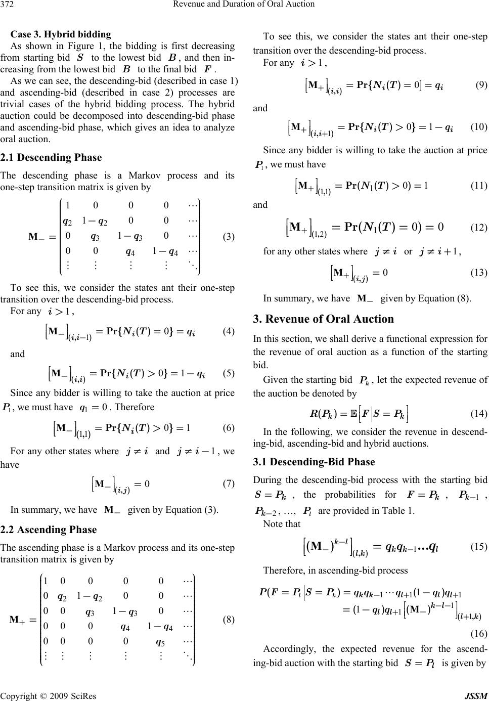

Revenue and Duration of Oral Auction 372
Case 3. Hybrid bidding
As shown in Figure 1, the bidding is first decreasing
from starting bid to the lowest bid , and then in-
creasing from the lowest bid to t he final bid .
S B
B F
As we can see, the descending-bid (described in case 1)
and ascending-bid (described in case 2) processes are
trivial cases of the hybrid bidding process. The hybrid
auction could be decomposed into descending-bid phase
and ascending-bid phase, which gives an idea to analyze
oral auction.
2.1 Descending Phase
The descending phase is a Markov process and its
one-step transition matrix is given by
22
33
44
1000
100
010
00 1
M




  
qq
qq
qq
-
æö
ç÷
ç÷
ç÷
ç÷
-
ç÷
ç÷
ç÷
-
ç÷ =ç÷
ç
ç
-
ç
ç
ç÷
ç÷
ç÷
èø
÷
÷
÷
÷
=
i
-
1
=
(3)
To see this, we consider the states ant their one-step
transition over the descending-bid process.
For any , 1i>
10M(, )Pr{( )}
ii
ii NT q
--
éù ==
êú
ëû (4)
and
01M(,) Pr{( )}
i
ii NT q
-
éù=>=
êú
ëû (5)
Since any bidder is willing to take the auction at price
, we must have . Therefore
1
P10q=
11 0M(,) Pr{( )}
i
NT
-
éù=>
êú
ëû (6)
For any other states where
j
i¹ and 1
j
i¹-, we
have
0M(, )ij
-
éù=
êú
ëû (7)
In summary, we have given by Equation (3 ). M-
2.2 Ascending Phase
The ascending phase is a Markov process and its one-step
transition matrix is given by
22
33
44
5
10 000
010 0
001 0
00 01
00 00
M






qq
qq
qq
q
+
æö
ç÷
ç÷
ç÷
ç÷ -
ç÷
ç÷
ç÷
-
ç÷
ç÷
=ç÷
ç÷
-
ç÷
ç÷
ç÷
ç
ç
ç
ç
ç
ç
è
To see this, we consider the states ant their one-step
transition over the descending-bid process.
For any ,
1i>
0M(,) Pr{()]
ii
ii NT q
+
é
ù==
êú =
ë
û (9)
and
101M(, )Pr{( )}
ii
ii NT q
++
é
ù=>=
êú -
ë
û (10)
Since any bidder is willing to take the auction at price
, we must have
1
P
11 10M(,) Pr(( ))NT
+1
é
ù=>
êú =
ë
û (11)
and
12 10 (, )Pr(( ))NT
+0
é
ù==
êú =
ë
û
M (12)
for any other states where
j
i¹ or 1
j
i¹+,
0M(, )ij
+
é
ù=
êú
ë
û (13)
In summary, we have given by Equation (8 ). M-
3. Revenue of Oral Auction
In this section, we shall derive a functional expression for
the revenue of oral auction as a function of the starting
bid.
Given the starting bid , let the expected revenue of
the auction be denoted by k
P
()
k
RPFS P
k
é
ù
==
ê
ú
ë
û
 (14)
In the following, we consider the revenue in descend-
ing-bid, ascending-bid and hybrid auctions.
3.1 Descending-Bid Phase
During the descending-bid process with the starting bid
, the probabilities for , ,
, …, are provided in Table 1.
k
SP=
k
P-
k
FP=1k P-
2l
Note that
P
1
(, )
() ...
kl
kk l
lk qq q
-
--
é
ù=
êú
ë
û
M (15)
Therefore, in ascending-bid process

÷
÷
÷
÷
÷
÷
ø
(8)
11 1
1
11
1
1M

(,)
() ()
()()
lkkkll l
kl
ll lk
PFPSPqqqq q
qq
-+ +
--
-
++
=== -
éù
=- êú
ëû
(16)
Accordingly, the expected revenue for the ascend-
ing-bid auction with the starting bid is given by
l
SP=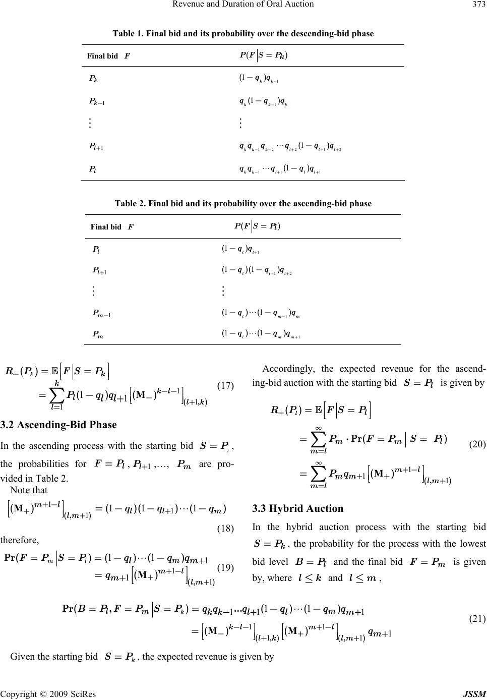

Revenue and Duration of Oral Auction373
Table 1. Final bid and its probability over the descending-bid phase
Final bid F()PFS P
k
=
k
P 1
1()
kk
qq
+
-
1k
P- 1
1()
kk
qqq
-
-k
1+
 
1l
P+ 1221 2
1()
kk klll
qq qqqq
--+++
-
l
P 11
1()
kkll l
qqqq q
-+
-
Table 2. Final bid and its probability over the ascending-bid phase
Final bid F()PFS P
l
=
l
P 1
1()
ll
qq
+
-
1l
P+ 12
11()( )
lll
qqq
++
--
 
1m
P- 1 11()( )
lm
qq
-
--
m
q
m m
P 1
11()( )
lm
qqq
+
--
1
1
1
11M(,
()
()()
kk
k
kl
llk
l
RPFSP
Pqq
ll
-
--
-+
=
éù
==
êú
ëû
éù
=-
+êú
ëû
å

)
)
(17)
3.2 Ascending-Bid Phase
In the ascending process with the starting bid ,
the probabilities for ,,…, are pro-
vided in Table 2.
l
SP=
l
FP=1l
P+m P
Note that
11
111 1M
(, )
()( )()(
ml m
ll
lm qq q
+-
++
+
éù
=- --
êú
ëû
(18)
therefore,
1
1
1
1
11
M

(, )
Pr()() ()
()
ml m
ml
lm
l
m
FPSP qqq
q+-
++
+
+
===--
éù
=êú
ëû
Accordingly, the expected revenue for the ascend-
ing-bid auction with the starting bid is given by
l
SP=
1
11
M(, )
()
Pr( )
()
ll
mm
ml
ml
mm lm
ml
RPFSP
PFPSP
Pq
¥
¥
+
=
+-
++ +
=
éù
==
êú
ëû
=⋅==
éù
=êú
ëû
å
å

l
(20)
3.3 Hybrid Auction
m
(19)
In the hybrid auction process with the starting bid
, the probability for the process with the lowest
bid level and the final bid is given
by, where and l,
k
SP=
l
BP=
lk£
m
FP=
m£
11
11
11 1
1
11
MM

(,)(,)
Pr(,)...() ()
() ()
kmm
l
klm l
lk lm
kk llm
m
BPFPSP qqqqqq
q
-- +-
-+
++
-+ +
+
== ==--
éùé ù
=êúê ú
ë
ûë û
(21)
Given the starting bid , the expected revenue is given by
k
SP=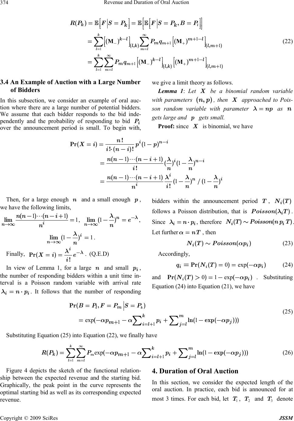

Revenue and Duration of Oral Auction 374
1
1
1
1
1
1
1
1
MM
MM
(, )(,)
(, )(,)
() ,
() ()
() ()
l
k
lml
k
lml
m
m
k
klm l
m
lk lm
klm l
mlk lm
kk
RPFS PFS PBP
Pq
Pq
¥
-+
==
¥
-+
==
+
+
-
+
-+-
+
+-
é
ù
éùéù
=====
êú
êúêú
ëûëû
ëû
éùé ù
=êúê ú
ëûë û
éùé ù
=êúê ú
ëûë û
åå
åå

(22)
3.4 An Example of Auction with a Large Number
of Bidders
In this subsection, we consider an example of oral auc-
tion where there are a large number of potential bidders.
We assume that each bidder responds to the bid inde-
pendently and the probability of responding to bid i P
over the announcement period is small. To begin with,
we give a limit theory as follows.
Lemma 1: Let X be a binomial random variable
with parameters , then approached to Pois-
son random variable with parameter as n
gets large and gets small.
(,np)X
np=
l
p
Proof: since is binomial, we have X
1
11
1
11
11


!
Pr()( )
!( )!
()()
()()
!
()()
()/(
!
ini
ini
ini
i
n
Xip p
ini
nnn i
inn
nnn i
in n
n
-
-
== -
⋅-
--+
=-
--+
=-
ll
ll l
)-
Then, for a large enough and a small enough ,
we have the following limits,
n p
11
1
()( )
lim i
n
nnni
n
¥
--+
=, 1lim ()n
ne
n
-
¥ -=
l
l,
11lim ()i
nn ¥ -=
l.
Finally, Pr() !
i
Xi e
i
-
== l
l. (Q.E.D)
In view of Lemma 1, for a large and small ,
the number of responding bidders within a unit time in-
terval is a Poisson random variable with arrival rate
. It follows that the number of responding
bidders within the announcement period T,
follows a Poisson distribution, that is .
Since , therefore .
Let further , then
ni p
i
np=⋅li
i
()
i
NT
()
i
n Tl
( )
ii
nnpT
Po
Po
)
pp -a
)
i
isso
isso
)
ii
i
np=⋅l
nT =a
N
Pr =
Pr(( )
i
NT
()NT~
(
ii
sson pa
0ex) (==
exp(p--a
()T
(qN
Poi~ (23)
Accordingly,
( )
iT (24)
and . Substituting
Equation (24) into Equation (21), we have
01)>=
1
1
exp 1
Pr( ,)
(ln( exp()))
km l
km
ij
il jl
m
BPFPSP
pp
=+ =
+
== =
=- -+--
åå
aa a p
j
(25)
Substituting Equation (25) into Equation (22), we finally have
11
1
exp 1()(ln(exp()))
k
m
lml
km
ki
il jl
m
RPP ppp
¥
== =+ =
+
=--+--
ååå å
aa a (26)
Figure 4 depicts the sketch of the functional relation-
ship between the expected revenue and the starting bid.
Graphically, the peak point in the curve represents the
optimal starting bid as well as its corresponding expected
revenue.
4. Duration of Oral Auction
In this section, we consider the expected length of the
oral auction. In practice, each bid is announced for at
most 3 times. For each bid, let , and denote
1
T2 T3 T

Revenue and Duration of Oral Auction375
050 100150200 250 300 350 40
0
0
5
10
15
20
25
30
35
40
45
Starting Price
Revenue
Revenue vs Starting Price
Optimal Revenue
Figure 4. Revenue vs starting bid
05 10 1520 25 30 35
2
4
6
8
10
12
14
16
18
Time
Bid din g p ri c e
Time Series of Bidding
Starting
Ending
Figure 5. Time evolution of a bidding process
the time length of the periods between the announce-
ments of the bid beginning, “going once” “going twice”
and “gone”, respectively. Let . For
example, when the auctioneer announces the bid , if
there is no response up to , that is , then
12
TTTT=++
P
10() i
NT =
3
2
3
i
1
T
the auctioneer announces “going once”; if there is still no
response up to , that is
then “going twice” will be announce; if there is no re-
sponse up to , that is , then
“gone” is announced. Figure 5 depicts a sample path of
the time evolution of the bidding process in term of a
step function.
1
TT+
12
TT++
120() i
NT T+=
0()
i
NT=T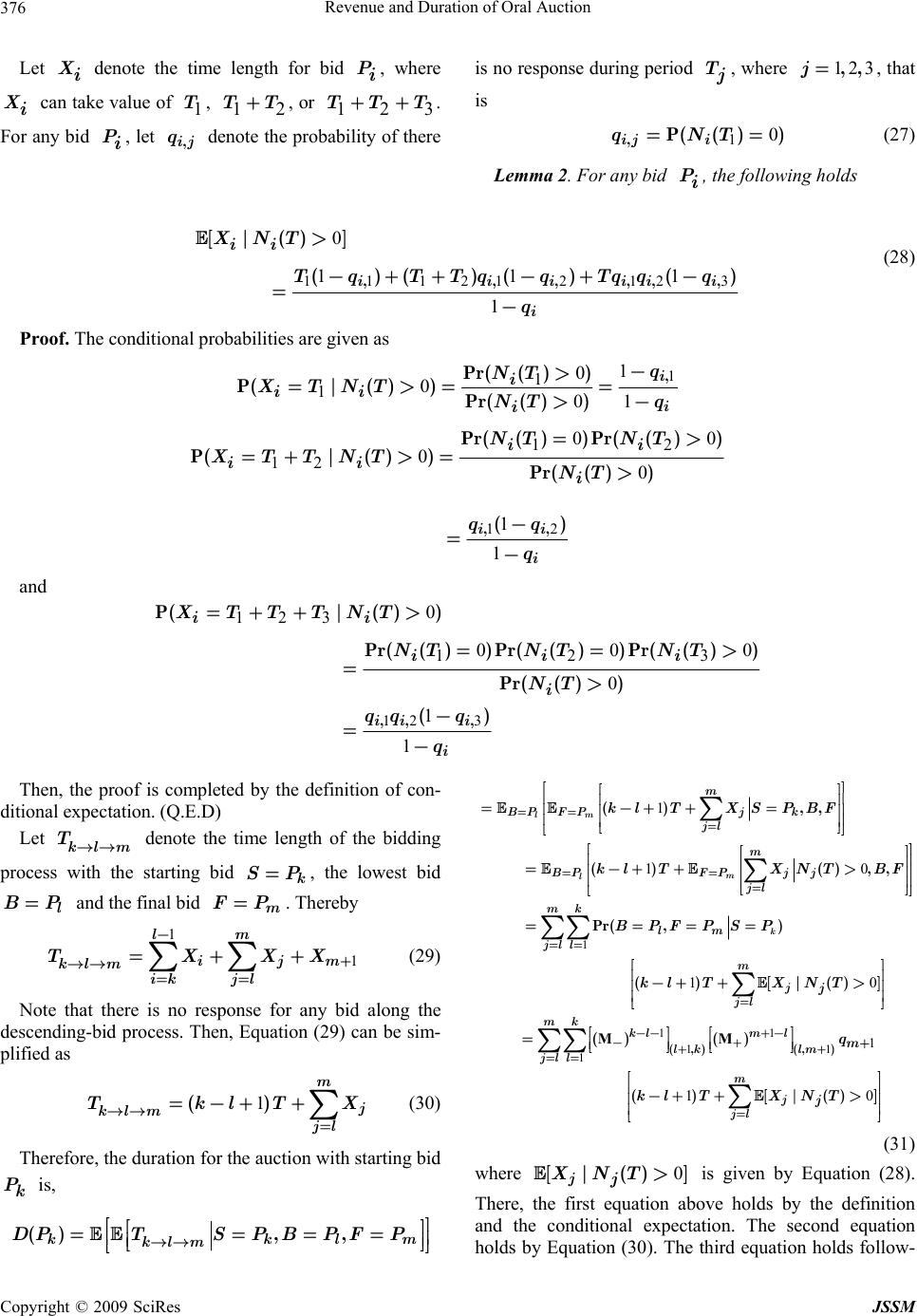

Revenue and Duration of Oral Auction 376
Let denote the time length for bid , where
can take value of , , or .
For any bid , let denote the probability of there
is no response during period XiP
i
12
TT+Xi1 T
,ij
1
TT+2 3 T+
P
iq
T
j
, where 12 3,,
j
=
=
, that
is
1
(
i
=0
,P() ) ij
qNT (27)
Lemma 2. For any bi d , the following holds P
i
11121212
0
11
1
,,,,,
[|() ]
()()( )(
iiiii
i
ii
XNT
TqTTqqTqqq
q
>
-++- +-
=-

3
1
,
)
i
(28)
Proof. The conditional probabilities are given as
1
1
11
0
001
,
Pr(( ))
P(|( ))Pr(( ))
i
i
i
ii
i
q
NT
XTNT NT q
-
>
=>= =
>-
12
12
12 00
00
1
1
,,
Pr(( ))Pr(())
P(|( ))Pr(( ))
()
ii
i
ii
ii i
NT NT
XTTNT NT
qq
q
=>
=+ >=>
-
=-
and
12 3
123
123
0
00
0
1
1
,, ,
P(|( ))
Pr( ())Pr( ())Pr( ())
Pr(( ))
()
ii i
i
ii
ii i
i
XTTTNT
NT NTNT
NT
qq q
q
=++>
==
=>
-
=-
0>
m
X
X
Then, the proof is completed by the definition of con-
ditional expectation. (Q.E.D)
Let denote the time length of the bidding
process with the starting bid , the lowest bid
and the final bid . Thereby
kl m
T
l
P
k
SP=
m
P=B=F
1
1
lm
ij
kl m
ik jl
TXX
-
+
 ==
=++
åå (29)
Note that there is no response for any bid along the
descending-bid process. Then, Equation (29) can be sim-
plified as
1()
m
j
kl m
jl
TklT
 =
=-++
å (30)
Therefore, the duration for the auction with starting bid
is,
k
P
(),, m
kk
kl m
DPTSPBPFP

é
é
===
ê
ê
ë
ë

1
1
1
1
10
10
M(,
() ,,
() (),,
Pr( ,)
() [|()]
()
m
l
m
l
k
m
BP FPjk
jl
m
BPFPjj
jl
mk
ml
jll
m
j
jl
kl
lk
j
klTXSPBF
kl TXNTBF
BPFPSP
kl TXNT
==
=
==
=
==
=
--
-+
é
ù
é
ù
êú
êú
=-++=
êú
êú
êú
êú
ëû
ëû
é
ù
éù
ê
ú
êú
=-++ >
ê
ú
êú
ê
ú
êú
ëû
ë
û
====
éù
êú
-+ +>
êú
êú
ëû
éù
=êú
ëû
å
å
åå
å



1
1
11
10
M
)(,)
()
() [|()]
mk
ml
lm
jll
m
j
jl
m
j
q
kl TXNT
+-
++
==
=
+
éù
êú
ëû
éù
êú
-+ +>
êú
êú
ë
û
åå
å
(31)
l
ù
ù
=
ú
ú
û
û
where is given by Equation (28).
There, the first equation above holds by the definition
and the conditional expectation. The second equation
holds by Equation (30). The third equation holds follow-
0[|()
jj
XNT>]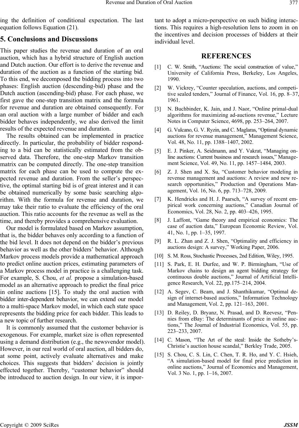

Revenue and Duration of Oral Auction377
ing the definition of conditional expectation. The last
equation follows Equation (21).
5. Conclusions and Discussions
This paper studies the revenue and duration of an oral
auction, which has a hybrid structure of English auction
and Dutch auction. Our effort is to derive the revenue and
duration of the auction as a function of the starting bid.
To this end, we decomposed the bidding process into two
phases: English auction (descending-bid) phase and the
Dutch auction (ascending-bid) phase. For each phase, we
first gave the one-step transition matrix and the formula
for revenue and duration are obtained consequently. For
an oral auction with a large number of bidder and each
bidder behaves independently, we also derived the limit
results of the expected revenue and duration.
The results obtained can be implemented in practice
directly. In particular, the probability of bidder respond-
ing to a bid can be statistically estimated from the ob-
served data. Therefore, the one-step Markov transition
matrix can be computed directly. The one-step transition
matrix for each phase can be used to compute the ex-
pected revenue and duration. From the seller’s perspec-
tive, the optimal starting bid is of great interest and it can
be obtained numerically by some basic searching algo-
rithm. With the formula for revenue and duration, we
may take their ratio to evaluate the efficiency of the oral
auction. This ratio accounts for the revenue as well as the
time, and thereby provides a comprehensive evaluation.
Our model is formulated based on Markov assumption,
that is, the bidder behaves only according to a function of
the bid level. It does not depend on th e bidder’s previous
behavior as well as the other bidders’ behavior. Although
Markov process models provide a mathematical approach
to predict online auction prices, estimating parameters of
a Markov process model in practice is a challenging task.
For example, S. Chou, et al. propose a simulation-based
model as an alternative approach to predict the final price
in online auctions [15]. To study the oral auction with
bidder inter-dependent behavior, we can extend our model
to a multi-space Markov model, in which each state space
represents the bidding price for each bidder. This leads to
a new topic of further research.
It is commonly assumed that the customer behavior is
exogenous. For example, market size is often represented
using a demand distribution (e.g., the newsvendor model).
However, in our real world of oral auction, all bidders do,
at some point, actively evaluate alternatives and make
choices. This suggests that bidders’ decision is jointly
effected together. Thereby, “customer behavior” should
be introduced to auction design. In our view, it is impor-
tant to adopt a micro-perspective on such biding interac-
tions. This requires a high-resolution lens to zoom in on
the incentives and decision processes of bidders at their
individual level.
REFERENCES
[1] C. W. Smith, “Auctions: The social construction of value,”
University of California Press, Berkeley, Los Angeles,
1990.
[2] W. Vickrey, “Counter speculation, auctions, and competi-
tive sealed tenders,” Journal of Finance, Vol. 16, pp. 8–37,
1961.
[3] N. Buchbinder, K. Jain, and J. Naor, “Online primal-dual
algorithms for maximizing ad-auctions revenue,” Lecture
Notes in Computer Science, 4698, pp. 253–264, 2007.
[4] G. Vulcano, G. V. Ryzin, and C . M aglaras , “O ptimal dynamic
auctions for revenue management,” Management Science,
Vol. 48, No. 11, pp. 1388–1407, 2002.
[5] E. J. Pinker, A. Seidmann, and Y. Vakrat, “Managing on-
line auctions: Current business and research issues,” Ma n a g e-
ment Science, Vol. 49, No. 11, pp. 1457–1484, 2003.
[6] Z. J. Shen and X. Su, “Customer behavior modeling in
revenue management and auctions: A review and new re-
search opportunities,” Production and Operations Man-
agement, Vol. 16, No. 6, pp. 713–728, 2009.
[7] K. Hendricks and H. J. Paarsch, “A survey of recent em-
pirical work concerning auctions,” Canadian Journal of
Economics, Vol. 28, No. 2, pp. 403–426, 1995.
[8] J. Laffont, “Game theory and empirical economics: The
case of auction data,” European Economic Review, Vol.
41, No. 1, pp. 1–35, 1997.
[9] R. L. Zhan and Z. J. Shen, “Optimality and efficiency in
auctions design: A survey,” Working Paper, 2006.
[10] S. M. Ross, Stochastic Processes, 2nd Edition, Wiley, 1995.
[11] S. Park, E. H. Durfee, and W. P. Birmingham, “Use of
Markov chains to design an agent bidding strategy for
continuous double auctions,” Journal of Artificial Intelli-
gence Research, Vol. 22, pp.175–214, 2004.
[12] A. Segev, C. Beam, and J. Shanthikumar, “Optimal de-
sign of internet-based auctions,” Information Technology
and Management, Vol. 2, pp. 121–163, 2001.
[13] D. Reiley, D. Bryanz, N. Prasad, and D. Reevesz, “Pen-
nies from eBay: The determinants of price in online auc-
tions,” The Journal of Industrial Economics, Vol. 55, pp.
223–233, 2007.
[14] C. Mason, “The Art of the steal: Inside the Sotheby’s-
Christie’s auction house scandal,” Berkley Trade, 2005.
[15] S. Chou, C. S. Lin, C. Chen, T. R. Ho, and Y. C. Hsieh,
“A simulation-based model for final price prediction in
online auctions,” Journal of Economics and Management,
Vol. 3 No. 1, pp. 1–16, 2007.