J. Service Science & Management, 2009, 2: 289-304
doi:10.4236/jssm.2009.24035 Published Online December 2009 (www.SciRP.org/journal/jssm)
289
How to React to the Subprime Crisis? - The Impact
of an Interest Rate Freeze on Residential Mortgage
Backed
Julia Hein, Thomas Weber
Department of Economics, University of Konstanz, Konstanz, Germany.
Received July 24, 2009; revised August 29, 2009; accepted October 3, 2009.
ABSTRACT
Several policy options have been discussed to mitigate the current subprime mortgage crisis. This paper analyses an
interest rate freeze on adjustable rate mortgages as one possible reaction. In particular, the implications on Residential
Mortgage Backed Securities (RMBS) are studied. We examine shifts in the underlying portfolio’s discounted cash flow
distributions as well as changes in the payment profile of RMBS-tranches. We show that the positive effects of a rate
freeze, e.g. less foreclosures and a stabilizing housing market, can outweigh the negative effect of lower interest income
such that investors might be better off.
Keywords: Interest Rate Freeze, Subprime Mortgages, Residential Mortgage, Backed Securities (RMBS)
1. Introduction
Starting in mid 2007, rising delinquency and foreclosure
rates in the US subprime mortgage market triggered a
severe financial crisis which spread around the world.
Although subprime mortgages, that were granted to bor-
rowers with weak credit record and often require less
documentation, only account for about 15 percent of all
outstanding US mortgages, they were responsible for
more than 50 percent of all mortgage loan losses in 2007
[1]. Most of the subprime losses were caused by high
foreclosure rates on hybrid adjustable rate mortgages
(ARM). These loans offer fixed initial interest rates at a
fairly low level, which are replaced by higher rates
linked to an interest rate index after two or three years1.
Thus, borrowers face a significant payment shock after
the interest reset which increases the probability of de-
linquencies. In previous years, rising real estate prices
and, thus, increasing home owner equity enabled mort-
gage associations to waive part of delinquent interest
payments in exchange for an increase in nominal value of
the mortgage or to renegotiate the mortgage. But during
the last year the trend in real estate prices has reversed in
many regions of the United States leading to “negative
equity” of many borrowers, i.e. to real estate values that
are lower than their outstanding debt. Consequently, de-
fault rates increased2.
Several policy options have been discussed to tackle
this crisis. The primary concern of policy makers was to
lower the financial burden of subprime borrowers and,
thus, to avoid further delinquencies and foreclosures
which in turn may stabilize house prices. The first policy
option is to provide direct financial support by disbursing
money to borrowers. In fact, this has been done in Feb-
ruary 2008 by means of the Economic Stimulus Act 2008,
which included tax rebates amounting from $300 to $600
per person. Whereas this policy action benefited every
tax payer and was not directly linked to the mortgage
loans, the Housing Bill of July 2008 was especially
targeted to subprime borrowers. Here a second policy
option was taken by providing state guarantees for mort-
gage loans. Thus, borrowers, who are close to foreclosure,
can refinance their loans at lower interest rates. Although
both policy actions certainly help to improve the situa-
tion of borrowers, the big drawback of these instruments
is that they are mainly financed by the tax payer who
cannot be blamed for the crisis. In contrast, mortgage
banks, who have been criticized for lax lending standards
[2], benefit from less defaults without accepting a re-
sponsibility.
1According to the IMF [1], $ 250 billion subprime mortgages are due
to reset in 2008.
2Mortgage loan
contracts in the United States often exclude personal
liability such that borrowers do not face any further financial
b
urden
when the
y
default.

How to React to the Subprime Crisis? - The Impact of an Interest Rate Freeze on Residential Mortgage Backed 290
A third policy option, which takes the banks’ failure
into account and which was proposed by the US gov-
ernment on December 6th, 2007, is an interest rate freeze.
This means that banks agree to waive (part of) the inter-
est rate step up on their ARMs. Although this proposal
did not become effective it raises the question whether
such an instrument may be better suited to mitigate the
current crisis. The aim of this paper is therefore to inves-
tigate the implications of an interest rate freeze.
Of course, subprime debtors will benefit from this
measure through reduced interest obligations. In contrast,
the effect on the lenders is not a priori clear. On the one
hand, they receive lower interest on a significant portion
of mortgage loans. On the other hand, they might benefit
in a twofold way. First, the number of defaults potentially
declines. Second, the average loss given default (LGD)
might be lower when house prices stabilize. Conse-
quently, there will be a shift in the repayment distribution
of the mortgage loan portfolio, which will be examined
in the paper.
But the impact of an interest-rate freeze is not limited
to borrowers and lenders. More than half of all subprime
mortgages that were granted in recent years were sold in
residential mortgage backed securities (RMBS). In these
RMBS transactions cash flows from the underlying
mortgage pool are allocated to tranches with different
seniority: several rated tranches and an equity tranche.
Due to a priority of payments scheme the equity tranche
absorbs most of the losses whereas the senior tranche
exhibits only low risk. Part of the RMBS tranches were
purchased by outside investors, i.e. foreign banks, non-
mortgage banks, insurance companies. As (part of) the
mortgage interest payments is used to cover losses that
otherwise might hit the rated tranches, RMBS investors
lose part of their loss protection following an interest rate
freeze. However, they also benefit from potentially lower
default losses. The combined effects lead to a realloca-
tion of cash flows and losses among investors which will
also be analysed in this paper.
Throughout the paper we look at three sample portfo-
lios: two subprime RMBS portfolios, from which one is
well diversified across regions and the other is geo-
graphically concentrated in regions that are later hit
hardest by the crisis, and one portfolio representing the
US mortgage market as a whole. First, we simulate the
stochastic repayments of each single mortgage loan using
Monte Carlo simulation. In particular, we use the re-
gional house price index as the systematic factor driving
the default rate as well as the loss given default. Addi-
tionally, we assume that each increase in the payment
obligations of a debtor, e.g. through an interest rate step
up, raises the default probability. Taking regional diversi-
fication into account, we aggregate the single payments
to get the repayment distributions of the mortgage loan
portfolios underlying the different RMBS transactions.
For all three portfolios we further assume a true-sale
RMBS transaction with four differently rated tranches
and an equity piece. We use a benchmark scenario with-
out crisis elements to calibrate the sizes and loss protec-
tion of the tranches to the respective rating. This scenario
includes an interest rate step-up after year two for non-
prime mortgage loans.
Subsequently, we derive the portfolio repayment dis-
tributions and the resulting tranche characteristics in a
crisis scenario that reflects the current situation in the
United States. In particular, the average house prices are
assumed to have decreased by six percent in the second
year of the RMBS transaction. As we show, the crisis
leads to a significant reduction of the expected dis-
counted cash flows of the respective portfolios ranging
from five percent for the US market portfolio to more
than 15 percent for the non-diversified subprime portfo-
lio. Hence, the equity piece often does not suffice to
cover the losses which means that the rated tranches need
to absorb a significant share of the portfolio loss. Conse-
quently, the risk characteristics of all tranches worsen as
compared to the benchmark case which makes severe
downgrades necessary as observed in the markets.
Starting from this crisis scenario we investigate the
impact of an interest rate freeze. We assume all sched-
uled interest rate step-ups to be waived which decreases
the claims on the RMBS portfolio. As subprime borrow-
ers evade this payment shock, foreclosure rates decrease.
First, we study only this direct effect of an interest rate
freeze. Our simulation results show that the net change in
expected portfolio payments is negative as is the effect
on most tranches. The consequences are not uniform for
all tranches however: the better the tranche, the less its
characteristics deteriorate. The senior tranches of the two
subprime RMBS even improve.
In the second case, we additionally include a posi-
tive ’second round’ effect on house prices. In particular,
the lower number of foreclosures takes pressure off the
housing market resulting such that the negative down-
ward trend is stopped. Given this combined impact, our
results indicate that the positive effects are able to (over-)
compensate for the loss due to the interest rate freeze. In
particular, all rated tranches benefit in this scenario as
compared to the crisis scenario. Therefore we conclude
that an interest rate freeze on mortgage loans does not
only improve the debtor situation, but might also render
investors in RMBS tranches better off at the expense of
the equity tranche which takes most of the crisis losses.
The remainder of this paper is structured as follows.
First we comment on related literature. Section 3 de-
scribes the set-up and calibration of our simulation model.
In Section 4, we analyse the effects of a mortgage crisis
on our sample mortgage portfolios and also on RMBS-
tranches backed by these portfolios. Furthermore, we
investigate the consequences of an interest rate freeze on

How to React to the Subprime Crisis? - The Impact of an Interest Rate Freeze on Residential Mortgage Backed291
portfolio and tranche characteristics. Section 5 concludes.
2. Literature Review
Our paper is closely related to the empirical study by
Cagan [3] analysing the impact of an interest rate reset in
adjustable rate mortgages (ARM). Based on a dataset of
ARMs originated between 2004 and 2006, he estimates
that 59% of these mortgages face a payment increase of
more than 25% after the initial period with low rates. He
anticipates that in total approximately 13% of adjust-
able-rate mortgages will default due to the interest rate
reset, which corresponds to 1.1 million foreclosures over
a total period of six to seven years. This increase in de-
fault rates is not equally distributed across all mortgages
but depends on the size of the interest rate step-up and
the loan-to-value ratio. Additionally, the author estimates
that each one-percent fall in national house prices causes
an additional 70,000 loans to enter reset-driven foreclo-
sure. Given a house price drop of 10% he projects that
more than 22% of ARMs will default due to the interest
rate reset. This underlines the impact of a policy reaction
to scheduled interest rate step-ups in the present market
environment.
Ashcraft and Schuermann [4] discuss the securitization
of subprime mortgages. First they provide a detailed
analysis of the key informational frictions that arise dur-
ing the securitization process and how these frictions
contributed to the current subprime crisis. They also doc-
ument the rating process of subprime mortgage backed
securities and comment on the ratings monitoring process.
They conclude that credit ratings were assigned to sub-
prime RMBS with significant error which has led to a
large downgrade wave of RMBS tranches in July 20073.
Several further research articles provide general in-
formation about subprime loans and the current mortgage
crisis. Chomsisengphet/Pennington-Cross [5] comment
on the evolution of the subprime market segment. In par-
ticular, some legal changes in the beginning of the 1980s,
which allowed to charge higher interest rates and higher
fees on more risky borrowers and which permitted to
offer adjustable rate mortgages, enabled the emergence
of subprime loans. The Tax Reform Act in 1986 allowing
interest deductions on mortgage loans made high loan-
to-value (LTV) ratios financially more rewarding and,
thereby, sub-prime mortgages more attractive. In the be-
ginning of the 1990s the increasing use of securitizations
as funding vehicles triggered rapid growth in the sub-
prime mortgage market. Between 1995 and 2006 the
volume in this market segment increased from $ 65 bil-
lion to more than $ 600 billion and also the share on the
total mortgage market significantly increased [6]. At the
same time the percentage of the outstanding subprime
loan volume being securitized went up from about 30%
to around 80% [2]. Dell’ Ariccia et al. [7] show that the
rapid expansion of the subprime market was associated
with a decline in lending standards. Additionally, they
find that especially in areas with higher mortgage securi-
tization rates and with more pronounced housing booms
lending standards were eased. Lower lending standards
can thus be identified as one reason for the subprime
mortgage crisis.
According to the IMF [1], subprime borrowers typi-
cally exhibit one or more of the following characteristics
at the time of loan origination: weakened credit histories
as indicated by former delinquencies or bankruptcies,
reduced repayment capacities as indicated by low credit
scores or high debt-to-income ratios and incomplete
credit histories. Given this very broad definition subpri-
me borrowers are not a homogeneous group. For exam-
ple, Countrywide Home Loans, Inc. distinguishes four
different risk categories of subprime borrowers4.These
subcategories may depend on the borrower’s FICO (Fair
Isaac Corporation) credit score, which is an indicator of
the borrowers credit history, the Loan-To-Value (LTV)
ratio of the mortgage loan, and the debt-to-income ratio5.
Analysing a data set of securitized loans from 1995 to
2004, Chomisengphet/Pennington-Cross [5] find strong
evidence for risk-based pricing in the subprime market.
In particular, interest rates differ according to credit sco-
res, loan grades and loan-to-value ratios.
Using a dataset of securitized subprime mortgages fro-
m 2001 to 2006, Demyanyk/Hemert [8] compare the
characteristics of different loan vintages in order to iden-
tify reasons for the bad performance of mortgages origi-
nated in 2006, which triggered the subprime mortgage
crisis. Their sample statistics show that the average FICO
credit score increased from 620 in 2001 to 655 in the
2006 vintage, which corresponds to the observation that
the market expanded in the less risky segment. During
the same period average loan size increased from $
151,000 to $ 259,000 whereas the average loan-to-value
(LTV) ratio at origin stayed approximately the same at
80%. Applying a logit regression model to explain de-
linquencies and foreclosure rates for the vintage 2006
mortgages, Demyanyk/Hemert [8] identify the low house
price appreciation as the main determinant for the bad
performance. Also Kiff/Mills [6], who comment on the
current crisis, see the slow down in house prices as the
main driver for the deterioration in 2006 vintage mort-
gage loans. Furthermore they emphasize that although
the average subprime borrower credit score increased
during the last years, also LTV and debt-to-income ratios
increased, which made the mortgages more risky.
Gerardi et al. [9] analyse a dataset of homeownership
experience in Massachusetts. They find that the 30 day
4
See www.cwbc.com or Chomsisengphet/Pennington-Cross [5] .
5
Kiff/Mills [6] classify a mortgage as subprime if the LTV is above
85% and/or t he debt-to-income ratio exceeds 55% .
3In fact there was a second downgrade wave in the beginning of 2008
on which the authors do not comment.

How to React to the Subprime Crisis? - The Impact of an Interest Rate Freeze on Residential Mortgage Backed 292
delinquency rate shows rather limited variance as it fluc-
tuates between 2 and 2.8 % of borrowers. Further, there
is no significant correlation to the change in house prices.
In contrast, they find a strong negative correlation be-
tween foreclosure rates and the house price index over
the whole sample period from 1989 to 2007. In particular,
Gerardi et al. [9] point out that the house price decline
starting in summer 2005 was the driver of rising foreclo-
sure rates in 2006 and 2007. These findings show that the
house price index drives the portion of delinquent mort-
gages that are foreclosed rather than the number of de-
linquencies themselves.
Estimating cumulative default probabilities they fur-
ther find that subprime borrowers default six times as
often as prime borrowers. This corresponds to Penning-
ton-Cross [10] who also compares the performance of
subprime to prime mortgage loans and finds that the lat-
ter are six times more likely to default and 1.3 times
more likely to prepay. Analysing the determinants of de-
fault he concludes that for both - prime and non-prime
loans - decreasing house prices as well as increasing
unemployment rates increase credit losses.
All these empirical studies indicate a strong relation-
ship between mortgage loan defaults and house price
appreciation in the subprime market. This corresponds to
the theoretical literature on mortgage loan default. Ac-
cording to option pricing theory a borrower, who is not
personally liable, should default when the associated put
option is in the money, e.g. when the mortgage debt ex-
ceeds the house value. Therefore we will use the house
price index as the main determinant of default in our
simulation model.
3. Model Set-Up
Our analysis is based on a cashflow simulation model.
Mortgage loans are more likely to default when they are
in “negative equity”, i.e. when the current real estate
value is lower than the outstanding debt. This event is
usually triggered by a downturn in the house price.
Therefore we use a macro factor representing the re-
gional house price index as the systematic determinant of
default. We assume the regional house price index to
have a nationwide and a regional component. The house
price at default further determines the loss incurred in a
distressed sale following a foreclosure.
Payment shocks due to interest rate resets can cause
additional foreclosures, especially when house prices
have already declined. We account for this by adding a
function depending on changes in payment obligations to
the idiosyncratic debtor component of our model.
3.1 Simulation Model
RMBS are usually backed by mortgage loans from dif-
ferent regions. This regional diversification reduces the
variance of the repayment distribution of the mortgage
portfolio and thereby helps to make the rated tranches
less risky. For each region we assume the regional house
price index (HPI) to be the main driver of the foreclosure
rate. Further, for each region k we decompose the per-
centage change of the HPI in year t into an overall posi-
tive long-term trend c and a deviation from this trend
driven by a nationwide factor Mt and an orthogonal re-
gional factor Bk,t :


,k
B
ktM tk
HPIc aM   ,t
= f (Mt , Mt−1, Bk,t , Bk,t−1 ) (1)
Unconditionally, Mt and Bk,t are assumed to be stan-
dard normally distributed. Empirical evidence suggests,
however, that house price changes display a strong posi-
tive autocorrelation6. Therefore we incorporate a first-
order autocorrelation of 0.5 for each factor. Thus, condi-
tional on Mt−1, Mt has a mean of 0.5· Mt−1 and a standard
deviation of 0.75 . The same holds for the regional
factors.
ρM and ρk account for correlations of house price
changes across and within regions. We calibrated the
nationwide and regional correlations to ρM = 0.1 and ρk =
0.2 and the scaling factor to a = 0.1. This implies uncon-
ditional standard deviations of 5.5% (3.7%) for annual
regional (nationwide) house price changes which is in
line with empirical evidence7. The unconditional mean
annual change of the HPI equals the long-term trend c on
both, the regional as well as the national level.
For the loans in the underlying mortgage pool we dis-
tinguish five debtor groups by credit quality: Prime,
Alt-A, Subprime 1, Subprime 2 and Subprime 3. These
groups can be interpreted as representing different ranges
of the FICO score and further borrower characteristics
like payment history and bankruptcies8.
The assumed expected default probabilities for the dif-
ferent debtor groups and maturities are shown in the cre-
dit curves in Table 1 in the appendix. The numbers cor-
respond to empirical evidence [9].
In each simulation run a path of annual group migra-
tions is computed for each loan in the portfolio. For
debtor i located in region k this path depends on a series
of latent migration variables Li,k,t , t = 1, . . . , 7. In this
respect our simulation model resembles a migration
6In an empirical study based on 15 OECD countries Englund an
d
Ioannidis [11] estimate an average first-order autocorrelation coef-
ficient of 0.45 .
7There exist
different house price indices for the US. For example,
Freddie Mac’s Con ven tional Mortgage Home Price Index (CMHPI-
Purchase Only) shows a standard deviation of 3.8% (nationwide)
and 5.2% regionally, since 1975.
8There exist no general classification scheme of mortgage loans
except for the distinction between Prime, Alt-A and Subprime.
Nevertheless it is common to further subdivide the subprime cate-
gory into several grades [5]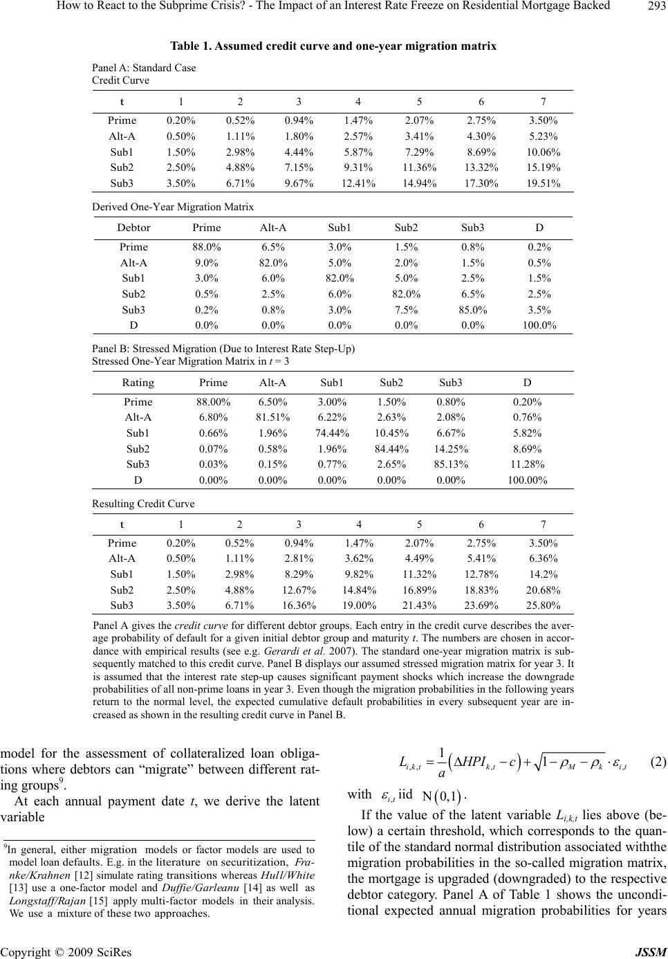
.

How to React to the Subprime Crisis? - The Impact of an Interest Rate Freeze on Residential Mortgage Backed 293
Table 1. Assumed credit curve and one-year migration matrix
Panel A: Standard Case
Credit Curve
t 1 2 3 4 5 6 7
Prime 0.20% 0.52% 0.94% 1.47% 2.07% 2.75% 3.50%
Alt-A 0.50% 1.11% 1.80% 2.57% 3.41% 4.30% 5.23%
Sub1 1.50% 2.98% 4.44% 5.87% 7.29% 8.69% 10.06%
Sub2 2.50% 4.88% 7.15% 9.31% 11.36% 13.32% 15.19%
Sub3 3.50% 6.71% 9.67% 12.41% 14.94% 17.30% 19.51%
Derived One-Year Migration Matrix
Debtor Prime Alt-A Sub1 Sub2 Sub3 D
Prime 88.0% 6.5% 3.0% 1.5% 0.8% 0.2%
Alt-A 9.0% 82.0% 5.0% 2.0% 1.5% 0.5%
Sub1 3.0% 6.0% 82.0% 5.0% 2.5% 1.5%
Sub2 0.5% 2.5% 6.0% 82.0% 6.5% 2.5%
Sub3 0.2% 0.8% 3.0% 7.5% 85.0% 3.5%
D 0.0% 0.0% 0.0% 0.0% 0.0% 100.0%
Panel B: Stressed Migration (Due to Interest Rate Step-Up)
Stressed One-Year Migration Matrix in t = 3
Rating Prime Alt-A Sub1 Sub2 Sub3 D
Prime 88.00% 6.50% 3.00% 1.50% 0.80% 0.20%
Alt-A 6.80% 81.51% 6.22% 2.63% 2.08% 0.76%
Sub1 0.66% 1.96% 74.44% 10.45% 6.67% 5.82%
Sub2 0.07% 0.58% 1.96% 84.44% 14.25% 8.69%
Sub3 0.03% 0.15% 0.77% 2.65% 85.13% 11.28%
D 0.00% 0.00% 0.00% 0.00% 0.00% 100.00%
Resulting Credit Curve
t 1 2 3 4 5 6 7
Prime 0.20% 0.52% 0.94% 1.47% 2.07% 2.75% 3.50%
Alt-A 0.50% 1.11% 2.81% 3.62% 4.49% 5.41% 6.36%
Sub1 1.50% 2.98% 8.29% 9.82% 11.32% 12.78% 14.2%
Sub2 2.50% 4.88% 12.67% 14.84% 16.89% 18.83% 20.68%
Sub3 3.50% 6.71% 16.36% 19.00% 21.43% 23.69% 25.80%
Panel A gives the credit curve for different debtor groups. Each entry in the credit curve describes the aver-
age probability of default for a given initial debtor group and maturity t. The numbers are chosen in accor-
dance with empirical results (see e.g. Gerardi et al. 2007). The standard one-year migration matrix is sub-
sequently matched to this credit curve. Panel B displays our assumed stressed migration matrix for year 3. It
is assumed that the interest rate step-up causes significant payment shocks which increase the downgrade
probabilities of all non-prime loans in year 3. Even though the migration probabilities in the following years
return to the normal level, the expected cumulative default probabilities in every subsequent year are in-
creased as shown in the resulting credit curve in Panel B.

,, ,,
11
iktktMkit
LHPIc
a



 (2)
model for the assessment of collateralized loan obliga-
tions where debtors can “migrate” between different rat-
ing groups9. with ,it

iid


0, 1.
At each annual payment date t, we derive the latent
variable If the value of the latent variable Li,k,t lies above (be-
low) a certain threshold, which corresponds to the quan-
tile of the standard normal distribution associated withthe
migration probabilities in the so-called migration matrix,
the mortgage is upgraded (downgraded) to the respective
debtor category. Panel A of Table 1 shows the uncondi-
tional expected annual migration probabilities for years
9In general, either
migration models or factor models are used to
model loan defaults. E.g. in the literature on securitization, Fra-
nke/Krahnen [12] simulate rating transitions whereas Hull/White
[13] use a one-factor model and Duffie/Garleanu [14] as well as
Longstaff/Rajan [15] apply multi-factor models in their analysis.
We use a mixture of these two a
pp
roac h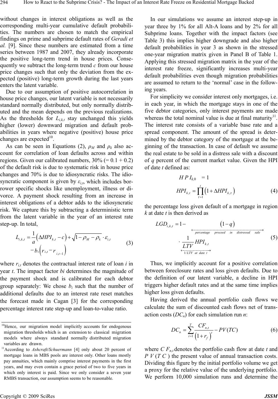es.

How to React to the Subprime Crisis? - The Impact of an Interest Rate Freeze on Residential Mortgage Backed 294
without changes in interest obligations as well as the
corresponding multi-year cumulative default probabili-
ties. The numbers are chosen to match the empirical
findings on prime and subprime default rates of Geradi et
al. [9]. Since these numbers are estimated from a time
series between 1987 and 2007, they already incorporate
the positive long-term trend in house prices. Conse-
quently we subtract the long-term trend c from our house
price changes such that only the deviation from the ex-
pected (positive) long-term growth during the last years
enters the latent variable.
Due to our assumption of positive autocorrelation in
house price changes, our latent variable is not necessarily
standard normally distributed, but only normally distrib-
uted and the mean depends on the previous realizations.
As the thresholds for Li,k,t stay unchanged this yields
higher (lower) downward migration and default prob-
abilities in years where negative (positive) house price
changes are expected10.
As can be seen in Equations (2), ρM and ρk also ac-
count for correlation of loan defaults across and within
regions. Given our calibrated numbers, 30% (= 0.1 + 0.2)
of the default risk is due to systematic risk in house price
changes and 70% is due to idiosyncratic risks. The idio-
syncratic component is given by εi,t, which includes bor-
rower specific shocks like unemployment, illness or di-
vorce. A payment shock resulting from an increase in
interest obligations of a debtor adds to the idiosyncratic
risk. We capture this by subtracting a deterministic term
from the latent variable in the year of an interest rate
step-up. In total,


,, ,,
,,1
11
iktktMk it
it iit
LHPIc
a
brr





(3)
where ri,t denotes the contractual interest rate of loan i in
year t. The impact factor bi determines the magnitude of
the payment shock and is calibrated for each debtor
group separately: We chose bi such that the number of
additional defaults due to an interest rate reset matches
the forecast made in Cagan [3] for the corresponding
percentage interest rate step-up and loan-to-value ratio.
In our simulations we assume an interest step-up in
year three by 1% for all Alt-A loans and by 2% for all
Subprime loans. Together with the impact factors (see
Table 3) this implies higher downgrade and also higher
default probabilities in year 3 as shown in the stressed
one-year migration matrix given in Panel B of Table 1.
Applying this stressed migration matrix in the year of the
interest rate freeze, significantly increases multi-year
default probabilities even though migration probabilities
are assumed to return to the ‘normal’ case in the follow-
ing years.
For simplicity we consider interest only mortgages, i.e.
in each year, in which the mortgage stays in one of the
five debtor categories, only interest payments are made
whereas the total nominal value is due at final maturity11.
The interest rate consists of a variable base rate and a
spread component. The amount of the spread is deter-
mined by the debtor category of the mortgage at the be-
ginning of the transaction. In case of default we assume
the real estate to be sold in a distress sale with a discount
of q percent of the current market value. Given the HPI
of date t defined as:
H P Ik,0 = 1

,
1
1
t
kt k

,
H
PI HPI

 

 (4)
the percentage loss given default of a mortgage in region
k at date t is then derived as

,,
,
1/
11
1
ikt
p
ercentageproceed in distressedsale
kt
LTVatdatet
LGD q
HPI
LTV



 
 (5)
Thus, we implicitly account for a positive correlation
between foreclosure rates and loss given defaults. Due to
the definition of our latent variable, a decline in HPI
triggers higher default rates and at the same time implies
higher loss given defaults.
Having derived the annual portfolio cash flows we
calculate the sum of discounted cash flows net of trans-
action costs (DCn) for each simulation run n:

,
1
()
1
Tnt
nt
tf
CF
DCPV TC
r



 (6)
10Hence, our
migration model implicitly accounts for endogenous
migration thresholds whic h is an extension to classical migration
models where always standard normally distributed mi gration
variables are dra wn.
11According to Ashcraft/Schuermann [4] only about 20 percent o
f
mortgage loans in MBS pools are interest only. Other loans mostly
pay annuities, which mainly comprise interest payments in the first
years, and may even contain a grace period of two to five years in
which only interest is paid. Since we only consider a seven year
RMBS transaction, our assumption seems to be reasonable.
where C Fn,t denotes the portfolio cash flow at date t and
P V (T C ) the present value of annual transaction costs.
Dividing this figure by the initial portfolio volume we get
a proxy for the relative value of the underlying portfolio.
We perform 10,000 simulation runs and determine the

How to React to the Subprime Crisis? - The Impact of an Interest Rate Freeze on Residential Mortgage Backed 295
distribution of this portfolio value as well as several sta-
tistics like mean, standard deviation and 99%-quantile.
Given the simulated portfolio cash flows at each an-
nual payment date we subsequently derive tranche pay-
ments. We assume that all losses (interest and principal)
are first covered by the excess spread of the transaction,
i.e. the difference between the interest income from the
underlying portfolio and the interest payments to the
rated tranches net of transaction costs, and then by re-
ducing the nominal value of the equity tranche. Further,
we assume the existence of a reserve account which
means that if the excess spread of one period is not wiped
out by period losses, the excess cash flow is collected in
this account earning the risk-free rate and providing a
cushion for future losses12. The holder of the equity
tranche does not receive any payments until maturity
when he receives the remaining cash flow of the transac-
tion. If the equity tranche has been reduced to zero due to
previous losses, the face value and subsequently the in-
terest claim of the lowest rated tranche is reduced to co-
ver the losses. If this tranche claim has already been red-
uced to zero, the next tranche is used to cover the losses, etc.
3.2 Sample Transactions
Throughout our analysis we consider three illustrative
sample portfolios: two subprime mortgage portfolios and
one representing the US mortgage market as a whole.
The former only include Alt-A and subprime mortgage
loans and differ with respect to their regional diversifica-
tion. The latter predominantly consist of prime (60%)
and Alt-A loans (25%). Five percent each fall in the three
subprime classes giving a total subprime share of 15%
for the portfolio which roughly resembles the subprime
portion in the US mortgage market. The explicit portfolio
compositions are given in Table 3 in the appendix.
Each mortgage is assumed to pay the risk-free rate,
which is assumed to be constant at 4%, plus a spread
Table 3. Portfolio characteristics and model assumptions
(‘Pacific’)
Subprime US Mortgage Market
Portfolio Portfolio
Portfolio:
Initial Volume $ 100,000,000 $ 100,000,000
Number of Mortgages 500 500
initial LTV 90% 90%
Share in Region
Pacific 20% (40%) 20%
New England 20% (40%) 20%
North Central 20% (20%) 20%
Atlantic 20% (-) 20%
South Central 20%(-) 20%
Share of Spreads (bps)
Prime - 60% 150
Alt-A 20% 25% 225
Subprime 1 30% 5% 300
Subprime 2 30% 5% 350
Subprime 3 20% 5% 400
0 Interest Rate (t = 0) 7.2% 6.0%
Interest Rate Step-Up (after 2 Years) Impact Factor (b)
Prime 0% 0% 0
Alt-A 1% 1% 15
Subprime 1-3 2% 2% 30
RMBS-Structure: Spreads (bps)
Tranches AAA AAA 30
AA AA 50
A A 80
BBB BBB 150
Equity Equity -
Transaction Costs 1% p.a. 1% p.a.
Maturity 7 years 7 years
This table presents the assumed portfolio compositions of our three sample portfolios as well as the assumed tranche structure. The two subprime
portfolios only differ in their regional diversification. The regional composition of the ’Pacific’ Subprime portfolio is given in brackets. The depicted
spreads are paid in addition to the risk-free rate of 4%.
12According to
Ashcraft/Schuermann [4] excess spread is at least captured for the first three to five years of a RMBS deal, which justifies the
assum
p
tion of a rese
r
v
e accoun
t
.

How to React to the Subprime Crisis? - The Impact of an Interest Rate Freeze on Residential Mortgage Backed 296
ranging between 150 and 400 basis points differentiated
by debtor category as shown in Table 3. Further we as-
sume that mortgage loans with an initial subprime (Alt-A)
rating include an interest rate step-up of 2% (1%) after
two years, i.e. all spreads are increased by 200 bps (100
bps) after this initial period13. The long-term trend is
house prices is assumed to be c = 3%, the loan-to-value
ratio at origin is 90% for each mortgage14 and the dis-
count in case of a distressed sale is q = 30%15. Geo-
graphically we differentiate five regions16: Pacific, Nor-
th Central (including Mountain), South Central, Atlantic
(middle and south) and New England. The first subprime
portfolio is concentrated in Pacific (40%) and New Eng-
land (40%), the regions to perform worst in the crisis, the
remaining 20% are North Ventral and Mountain. The
other two portfolios are well diversified across all regions.
First we simulate payments for the portfolios in the
benchmark case, i.e. without any crisis. In year 3 the la-
tent variable Li,k,t for each loan is stressed by the impact
factor of the current debtor category times the scheduled
interest rate step-up which causes an increase in expected
cumulative default rates as shown in Panel B of Table 1.
Since there is no step-up for prime loans, the expected
default rates of these loans stay the same.
Columns 3 in Tables 4, 5 and 6 present some statistics
describing the port-folios’ repayment distribution. In the
benchmark case the expected value of discounted cash
flows (net of transaction costs) clearly exceeds the nom-
inal value for all three portfolios. The exceedance equals
more than two times the standard deviation of discounted
cash flows. For the subprime portfolios the average value
of the discounted portfolio payment stream after deduct-
ing all fees is 113.4% of the initial face value. Since we
use the risk-free rate for discounting, this number corre-
sponds to a yearly average premium of 1.9% on top of
the risk-free rate. The standard deviations over seven
years are 5% for the well diversified portfolio and 5.6%
for the concentrated one. In case of the representative
portfolio the expected discounted value in the benchmark
case is 105.5%, yielding an average premium of 0.8%
p.a., with a standard deviation of 2.4% over seven years.
Subsequently, we simulate payments of three residen-
tial mortgage backed security (RMBS) transactions wh-
ich are backed by the sample portfolios and have a ma-
turity of seven years. We assume that four rated tranches
AAA, AA, A and BBB are issued that earn the usual
market spreads as shown in Table 3. Additionally, we
assume annual transaction costs of 1%, which are paid
before any interest payment to the tranches.
We calibrate tranche sizes such that their default pro-
babilities in the bench-mark scenario are roughly in line
with the historical averages given by Standard & Poor’s
for the respective rating classes and a seven year maturity.
The resulting tranche sizes are also shown in Tables 4, 5
and 617. The calibrated tranche structures correspond to
typical RMBS structures observed in the market [4]. As
can be seen the AAA tranches is smallest and the equity
tranche is highest for the ’Pacific’ subprime portfolio,
which is due to a worse regional diversification.
4. Analysis of Mortgage Crisis
4.1 Crisis Scenario
Having calibrated our model to the benchmark case we
now turn to modeling the crisis scenario. In particular we
assume that the sample transaction was set-up two years
ago (e.g. second quarter of 2006) with tranche sizes as
derived before. The nationwide and regional house price
index changes are set to match Freddie Mac’s Conven-
tional Mortgage Home Price Index18. In the first year of
the transaction, the increase in national house prices
slowed down to 2.6%, in the second year there was a
downturn of 6%. Regionally, Pacific developed worst
with a cumulated two year decrease of 15% in house
prices, whereas South Central saw an appreciation of 6%.
Table 2 shows all regional trends and the corresponding
nationwide and regional macro factors. Figure 1 shows
13This step-up is assumed to be fixed at loan origination and is inde-
pendent of possible downward migrations until the reset date.
14Gerardi et al. [9] report a mean LTV ratio of 83% and a median o
f
90% in the last three years.
15Pennington-Cross [16] provides a survey study on the discount in
case of a distressed sale and finds that foreclosed property appreci-
ates on average 22% less than the area average appreciation rate.
Given that foreclosures also lead to additional costs, we will assume
a discount of 30% on the current market value in our simulation
analysis. Cagan [3] also states that foreclosure discounts of 30% are
quite usual.
16We followed the regions defined in Freddie Mac’s Conventional
Mortgage Home Price Index but pooled some neighbouring regions.
17A slightly different tranche structure would arise when using the
expected loss rating from Moody’s. But it should be noted that
tranches with the same rating have nearly the same expected losses
in our benchmark case.
18Our reference index is the ’
p
urchase onl
y
’ index.
Figure 1. Expected HPI for different scenarios
This figure shows the expected development of the House Price Index
(HPI) averaged over our five regions for different simulation scenarios:
In the benchmark case a long-term house price growth of 3% p.a. is
assumed. The crisis scenario is set by fixing macrofactor realisations in
the first two years (see Table 1) which cause a severe decline in house
prices. Departing from this crisis scenario the positive feedback sce-
nario assumes that there is no autocorrelation between years 2 and 3,
such that house prices recover faster from the crisis. The scenarios
Robustness 1 and 2 assume a weaker house price stabilization as the
utocorrelation is only reduced by a half or one fourth, respectively. a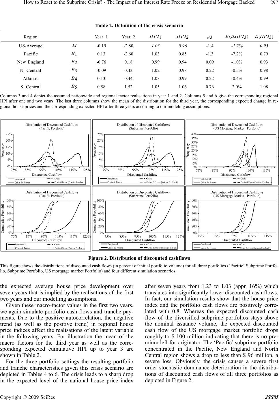

How to React to the Subprime Crisis? - The Impact of an Interest Rate Freeze on Residential Mortgage Backed297
Table 2. Definition of the crisis scenario
Region Year 1 Year 2 H P
I
1
H P I
2
µ
3
E (∆ H P I
3
) E [ H P I
3
]
US-Av erage M -0.19 -2.80 1.03 0.96 -1.4 -1.2% 0.95
Pacific
B
1
0.13 -2.60 1.03 0.85 -1.3 -7.2% 0.79
New England
B
2
-0.76 0.18 0.99 0.94 0.09 -1.0% 0.93
N. Cen tral
B
3
-0.09 0.43 1.02 0.98 0.22 -0.5% 0.98
Atlantic
B
4
0.13 0.44 1.03 0.99 0.22 -0.4% 0.99
S. Cen tral
B
5
0.58 1.52 1.05 1.06 0.76 2.0% 1.08
Columns 3 and 4 depict the assumed nationwide and regional factor realisations in year 1 and 2. Columns 5 and 6 give the corresponding regional
HPI after one and two years. The last three columns show the mean of the distribution for the third year, the corresponding expected change in re-
gional house prices and the corresponding expected HPI after three years according to our modeling assumptions.
Figure 2. Distribution of discounted cashflow s
This figure shows the distributions of discounted cash flows (in percent of initial portfolio volume) for all three portfolios (‘Pacific’ Subprime Portfo-
lio, Subprime Portfolio, US mortgage market Portfolio) and four different simulation scenarios.
the expected average house price development over
seven years that is implied by the realisations of the first
two years and our modelling assumptions.
Given these macro-factor values in the first two years,
we again simulate portfolio cash flows and tranche pay-
ments. Due to the positive autocorrelation, the negative
trend (as well as the positive trend) in regional house
price indices affect the realisations of the latent variable
in the following years. For illustration the mean of the
macro factors for the third year as well as the corre-
sponding expected cumulative HPI up to year 3 are
shown in Table 2.
For the three portfolio settings the resulting portfolio
and tranche characteristics given this crisis scenario are
depicted in Tables 4 to 6. The crisis leads to a sharp drop
in the expected level of the national house price index
after seven years from 1.23 to 1.03 (appr. 16%) which
translates into significantly lower discounted cash flows.
In fact, our simulation results show that the house price
index and the portfolio cash flows are positively corre-
lated with 0.8. Whereas the expected discounted cash
flow of the diversified subprime portfolios stays above
the nominal issuance volume, the expected discounted
cash flow of the US mortgage market portfolio drops
roughly to $ 100 million indicating that there is no pre-
mium left for originator. The ‘Pacific’ subprime portfolio
concentrated in the Pacific, New England and North
Central region shows a drop to less than $ 96 million, a
severe loss. Obviously, the crisis causes a severe first
order stochastic dominance deterioration in the distribu-
tions of discounted cash flows of all three portfolios as
depicted in Figure 2.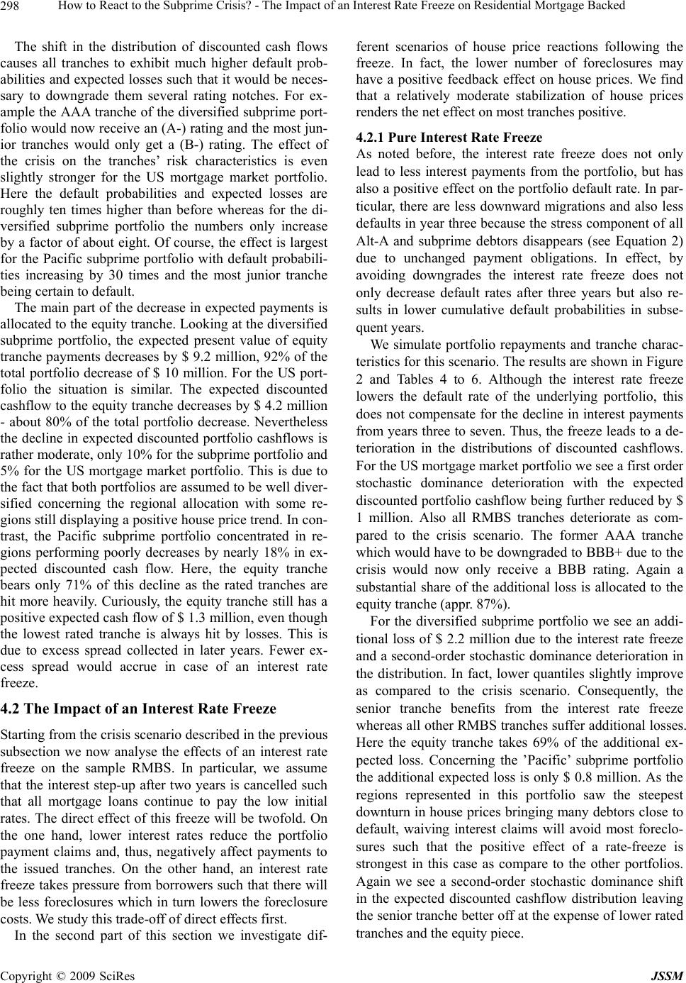

How to React to the Subprime Crisis? - The Impact of an Interest Rate Freeze on Residential Mortgage Backed 298
The shift in the distribution of discounted cash flows
causes all tranches to exhibit much higher default prob-
abilities and expected losses such that it would be neces-
sary to downgrade them several rating notches. For ex-
ample the AAA tranche of the diversified subprime port-
folio would now receive an (A-) rating and the most jun-
ior tranches would only get a (B-) rating. The effect of
the crisis on the tranches’ risk characteristics is even
slightly stronger for the US mortgage market portfolio.
Here the default probabilities and expected losses are
roughly ten times higher than before whereas for the di-
versified subprime portfolio the numbers only increase
by a factor of about eight. Of course, the effect is largest
for the Pacific subprime portfolio with default probabili-
ties increasing by 30 times and the most junior tranche
being certain to default.
The main part of the decrease in expected payments is
allocated to the equity tranche. Looking at the diversified
subprime portfolio, the expected present value of equity
tranche payments decreases by $ 9.2 million, 92% of the
total portfolio decrease of $ 10 million. For the US port-
folio the situation is similar. The expected discounted
cashflow to the equity tranche decreases by $ 4.2 million
- about 80% of the total portfolio decrease. Nevertheless
the decline in expected discounted portfolio cashflows is
rather moderate, only 10% for the subprime portfolio and
5% for the US mortgage market portfolio. This is due to
the fact that both portfolios are assumed to be well diver-
sified concerning the regional allocation with some re-
gions still displaying a positive house price trend. In con-
trast, the Pacific subprime portfolio concentrated in re-
gions performing poorly decreases by nearly 18% in ex-
pected discounted cash flow. Here, the equity tranche
bears only 71% of this decline as the rated tranches are
hit more heavily. Curiously, the equity tranche still has a
positive expected cash flow of $ 1.3 million, even though
the lowest rated tranche is always hit by losses. This is
due to excess spread collected in later years. Fewer ex-
cess spread would accrue in case of an interest rate
freeze.
4.2 The Impact of an Interest Rate Freeze
Starting from the crisis scenario described in the previous
subsection we now analyse the effects of an interest rate
freeze on the sample RMBS. In particular, we assume
that the interest step-up after two years is cancelled such
that all mortgage loans continue to pay the low initial
rates. The direct effect of this freeze will be twofold. On
the one hand, lower interest rates reduce the portfolio
payment claims and, thus, negatively affect payments to
the issued tranches. On the other hand, an interest rate
freeze takes pressure from borrowers such that there will
be less foreclosures which in turn lowers the foreclosure
costs. We study this trade-off of direct effects first.
In the second part of this section we investigate dif-
ferent scenarios of house price reactions following the
freeze. In fact, the lower number of foreclosures may
have a positive feedback effect on house prices. We find
that a relatively moderate stabilization of house prices
renders the net effect on most tranches positive.
4.2.1 Pure Interest Rate Freeze
As noted before, the interest rate freeze does not only
lead to less interest payments from the portfolio, but has
also a positive effect on the portfolio default rate. In par-
ticular, there are less downward migrations and also less
defaults in year three because the stress component of all
Alt-A and subprime debtors disappears (see Equation 2)
due to unchanged payment obligations. In effect, by
avoiding downgrades the interest rate freeze does not
only decrease default rates after three years but also re-
sults in lower cumulative default probabilities in subse-
quent years.
We simulate portfolio repayments and tranche charac-
teristics for this scenario. The results are shown in Figure
2 and Tables 4 to 6. Although the interest rate freeze
lowers the default rate of the underlying portfolio, this
does not compensate for the decline in interest payments
from years three to seven. Thus, the freeze leads to a de-
terioration in the distributions of discounted cashflows.
For the US mortgage market portfolio we see a first order
stochastic dominance deterioration with the expected
discounted portfolio cashflow being further reduced by $
1 million. Also all RMBS tranches deteriorate as com-
pared to the crisis scenario. The former AAA tranche
which would have to be downgraded to BBB+ due to the
crisis would now only receive a BBB rating. Again a
substantial share of the additional loss is allocated to the
equity tranche (appr. 87%).
For the diversified subprime portfolio we see an addi-
tional loss of $ 2.2 million due to the interest rate freeze
and a second-order stochastic dominance deterioration in
the distribution. In fact, lower quantiles slightly improve
as compared to the crisis scenario. Consequently, the
senior tranche benefits from the interest rate freeze
whereas all other RMBS tranches suffer additional losses.
Here the equity tranche takes 69% of the additional ex-
pected loss. Concerning the ’Pacific’ subprime portfolio
the additional expected loss is only $ 0.8 million. As the
regions represented in this portfolio saw the steepest
downturn in house prices bringing many debtors close to
default, waiving interest claims will avoid most foreclo-
sures such that the positive effect of a rate-freeze is
strongest in this case as compare to the other portfolios.
Again we see a second-order stochastic dominance shift
in the expected discounted cashflow distribution leaving
the senior tranche better off at the expense of lower rated
tranches and the equity piece.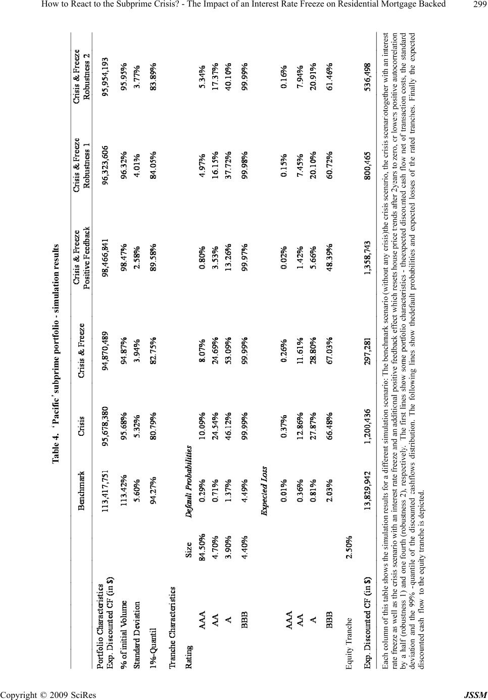

How to React to the Subprime Crisis? - The Impact of an Interest Rate Freeze on Residential Mortgage Backed 299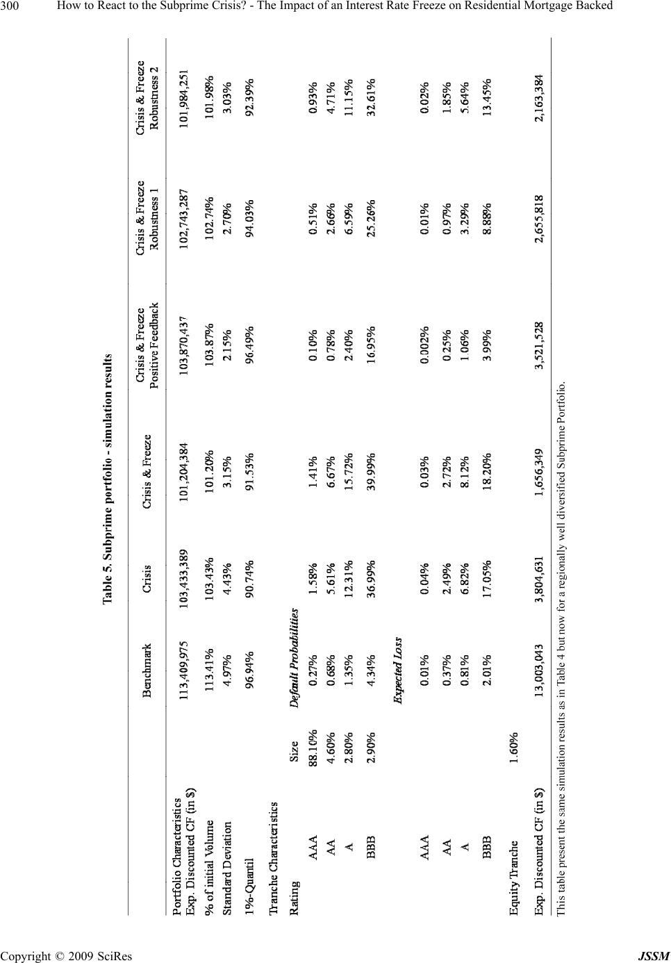

How to React to the Subprime Crisis? - The Impact of an Interest Rate Freeze on Residential Mortgage Backed 300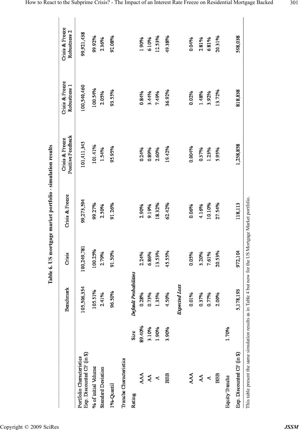

How to React to the Subprime Crisis? - The Impact of an Interest Rate Freeze on Residential Mortgage Backed301

How to React to the Subprime Crisis? - The Impact of an Interest Rate Freeze on Residential Mortgage Backed 302
4.2.2 Inter est R ate Fr eeze and Posi tive Fee dback E ffect
As shown in the previous subsection, the first round ef-
fects of an interest rate freeze are not sufficient to attenu-
ate the crisis. Yet a decrease in foreclosure rates may take
pressure off the housing market such that the negative
trend in the regional house prices is mitigated19. This in
turn will lead to a positive effect on subsequent foreclo-
sure rates.
In the previous scenarios, persistent trends in the house
price index are implemented by positive autocorrelation
in the house price index. Therefore the downturn in years
one and two leads to an expected downturn in year three,
i.e. the conditional mean of the variable describing
changes in the house price index is negative. Combined
with the regional components, this yields expected house
price changes of between -7.2% and 2.0% for the respec-
tive regions, nationwide -1.2% (see Table 2) which is
substantially below the long-term mean of 3%. We now
assume these negative trends to be stopped by the interest
intervention. In effect, expected house price apprecia-
tions rise to the long-term trend of 3% for region 1 (Pa-
cific) and up to 6.4% for region 5 (South Central) in year
3. We implement this by excluding the autocorrelation
effects from year two to year three in the nationwide
factor as well as in all regions with negative factor re-
alization in year 2. In total, the average HPI stabilizes by
four percent in year three. Feedback effects in subsequent
years result in an average HPI that by the end of year
seven is appr. 11 percent higher than in the crisis scenario,
as shown in Figure 1. The results for the portfolios are
displayed in Figure 2 and Tables 4 to 6.
For both subprime portfolios the expected discounted
cashflow exceeds the value in the crisis scenario without
an interest rate freeze. Comparing the cumulative ex-
pected discounted cash flow distributions this positive
feedback scenario second-order stochastically dominates
the crisis scenario with all lower quantiles being substan-
tially improved. Consequently, all rated RMBS tranches
benefit concerning their default probabilities and also
their expected losses. Given the diversified subprime
portfolio the AAA and the AA tranche perform as well as
in the benchmark scenario without crisis meaning that no
downgrade would be necessary. The costs of the interest
rate freeze are completely borne by the owner of the eq-
uity tranche.
The US mortgage market portfolio loses less interest
payments due to the interest rate freeze as prime mort-
gage loans representing 60% of the portfolio do not in-
corporate an interest step-up. Here, the positive effect of
stopping the house price decline overcompensates the
foregone interest resulting in higher expected discounted
cash flow compared to the crisis scenario. All tranches
including the equity tranche profit with higher tranches
benefiting most. This is due to a more narrow distribution
of losses. Compared to the crisis we again observe a
second order stochastic dominance shift in cumulative
repayments.
Summarizing, our results indicate that an interest rate
freeze may help to alleviate the current crisis. Even
though RMBS tranche investors lose a significant portion
of their loss protection, this deterioration may be over-
compensated by improvements in mortgage payments
due to lower foreclosure rates and a positive feedback
effect in the housing market. For all three portfolios we
derive positive net effects on all rated RMBS tranches as
compared to the crisis scenario. The higher the tranche,
the more it improves. Especially, the AAA tranche bene-
fits from the rate freeze. Thus, the RMBS market will
benefit from an interest rate freeze which can induce
positive spill over effects on other markets. In particular,
markets for other structured instruments containing
RMBS tranches may stabilize. Especially, special in-
vestment vehicles backing their commercial paper fund-
ing with senior RMBS tranches may recover.
4.3 Robustness Checks
1) Assumptions concerning House Price Developments
Our previous results depend on several assumptions
concerning house price developments which are moti-
vated by empirical findings. We set the crisis scenario to
match house price developments in the main US regions
during the last two years. When discussing the positive
feedback effect of an interest rate freeze we had to make
a specific assumption concerning house price stabiliza-
tion. Naturally, other house price reactions are also pos-
sible.
As robustness checks we derive portfolio and tranche
repayments for less favorable assumptions concerning
house price stabilization. In particular we assume the
negative house price trend only to be partially offset by
the interest rate freeze. Instead of zero autocorrelation in
year three increasing the average house price index by
four percent compared to the crisis situation, we now
assume that only half (one fourth) of this effect is real-
ised. Figure 1 shows the expected average house price
development for these two scenarios. Tables 4 to 6 dis-
play the tranche and portfolio characteristics for these
additional scenarios.
As can be seen, a more moderate stabilization of two
percent in year three (translating into 5.5 percentage
points until year seven) is sufficient to substantially im-
prove all rated RMBS tranches (see Robustness 1 ). Even
a stabilization of only one percent in year three (incresing
to 2.7 percent in year seven) leaves the rated tranches
slightly better off than in the crisis scenario (see Robust-
ness 2 ).
19Cagan [3] finds significant additional foreclosure discounts in re-
gions with high foreclosure rates. This indicates limited buyer ca-
pacities unable to absorb the excess supply without additional dis-
counts.

How to React to the Subprime Crisis? - The Impact of an Interest Rate Freeze on Residential Mortgage Backed303
Given these results we conclude that the qualitative
results are quite stable towards changes in the assump-
tion of house price stabilization: Due to lower excess
spread, the payments to the equity tranche will be re-
duced the most and due to lower probabilities of high
losses the highest rated tranche will profit most from an
interest rate freeze. Even for modest house price reac-
tions the net effect of the freeze is positive.
2) Assumptions concerning RMBS-Structure
A further assumption which needs to be critically re-
viewed is our assumption concerning the payment wa-
terfall for our RMBS tranches. In the previous simula-
tions we always assumed the existence of an unlimited
reserve account, which means that the holder of the eq-
uity tranche only receives payments at final maturity and
that at each annual payment dates all excess cash flows
are placed in an extra account which can be used to cover
future losses. In fact other reserve account specifications
are possible, e.g. a capped reserve account, where all
excess cash flows above this cap are paid out to the
holder of the equity piece periodically, or even a structure
without any reserve account, in which the holder of the
equity tranche receives all excess cash flow at each pay-
ment date.
This assumption mainly influences the calibration of
tranche sizes in the benchmark case. In particular, a
structure without a reserve account will lead to a much
smaller AAA tranche a bigger equity tranche. In this case
the effect of the interest rate freeze is less pronounced
since the tranche sizes are already calibrated to provide a
better protection against interest losses. Nevertheless, the
qualitative effects stay the same with the difference that
now an even more moderate house price stabilization is
sufficient to make all rated tranches better off than in the
pure crisis scenario.
4.4 Other Policy Options
1) Interest rate cuts
Throughout the paper we assumed that the risk-free
interest rate on top of which credit spreads are paid stays
the same over seven years. In fact the crisis might lead to
a cut in this reference rate. Looking at the repayments of
the mortgage loans analysed in this paper lowering the
reference rate would have a positive effect. Thus, interest
rate cuts are an additional policy option worth examining.
However, discussing the macroeconomic consequences
of interest rate cuts is beyond the scope of this paper.
2) Housing Bill
For mortgage debtors the effects of the proposed in-
terest rate freeze are comparable to the sought impact of
the Housing Bill of July 2008. Here, state guarantees
help troubled borrowers to refinance at lower rates. The
key difference between the two policy options is on the
lender side. With the interest rate freeze, mortgage banks
and equity tranche holders bear the potential costs.
Looking at a portfolio of mortgage loans the state guar-
antee included in the Housing Bill adds a large state
owned first loss position, irrespective of the portfolio
being securitized. Compared to our simulation results
above, lenders, all rated tranches and especially the eq-
uity tranche would profit at the tax payers expense.
5. Conclusions
The discussed interest rate moratorium for subprime
mortgages is one option to tackle the current crisis. It is
an agreement between two parties - the U.S. government
and the originating banks - that affects two different third
parties: the mortgage debtors and investors in RMBS
tranches. The first group will unambiguously profit from
an interest rate freeze. Some of their payment obligations
are waived, thus they might avoid default. Additionally,
they benefit from a stabilizing housing market.
The effect on RMBS-tranches is more ambiguous.
First, we show that the pure interest rate freeze decreases
the portfolio payment stream’s expected value by one to
2.2 percent, depending on portfolio composition. The
vast majority of this decrease is borne by the equity
tranche. Default probability and expected loss of rated
tranches only slightly deteriorate as compared to the cri-
sis scenario with senior tranches even being better off.
Second, we take into account that the interest rate freeze
may have a positive second round effect as a reduction in
foreclosures takes pressure off the housing market. In
this case we find that already a very moderate mitigation
of the house price downturn yields a positive net effect
on all rated tranches. A stabilization of one percent in
year three leaves all tranches in each of our three sample
transactions better off (compared to the crisis scenario
without policy reaction). For the holder of the equity
tranche, the situation is different. Looking at the average
of the three sample RMBS a four percent stabilization in
house prices is needed for him to slightly benefit from
the interest rate freeze. Thus, should the US government
and loan and savings associations decide on an interest
moratorium on adjustable rate subprime mortgages, this
would probably not come at the expense of the RMBS
investors as a third party. If additional losses occur they
are borne by originators and equity tranche investors. As
these parties are the ones in charge of the criticized lend-
ing standards we argue that reconsidering this policy op-
tion is worth wile.
REFERENCES
[1] International Monetary Fund, Global Financial Stability
Report, Washington DC, April 2008.
[2] Keys, J. Benjamin, T. Mukherjee, A. Seru, and V. Vig,
“Did securitization lead to lax screening? Evidence from
Subprime Loans,” Working Paper, 2008.
[3] Cagan, L. Christopher, “Mortgage payment reset: The issue

How to React to the Subprime Crisis? - The Impact of an Interest Rate Freeze on Residential Mortgage Backed 304
and impact,” First American CoreLogic, March 19, 2007.
[4] Ashcraft, B. Adam, and T. Schuermann, “Understanding
the securitization of subprime mortgage credit,” Federal
Reserve Bank of New York Staff Reports, No. 318, 2008.
[5] Chomsisengphet, Souphala and A. Pennington-Cross,
“The evolution of the subprime mortgage market,” Fed-
eral Reserve Bank of St. Louis Review, Vol. 88, No. 1, pp.
31–56, 2006.
[6] Kiff, John and P. Mills, “Money for nothing and checks
for free: Recent developments in U.S. subprime mortgage
markets,” Working Paper, International Monetary Fund,
07/188, 2007.
[7] G. Dell’ Ariccia, D. Igan, and L. Laeven, “Credit booms
and lending standards: Evidence from the subprime
mortgage market,” Working Paper, 2008.
[8] Demyanyk, Yuliya and Otto Van Hemert, “Understanding
the subprime mortgage crisis,” Working Paper FRB St.
Louis and NYU Stern, 2007.
[9] Gerardi, Kristofer, A. H. Shapiro and P. S. Willen: “Sub-
prime outcomes: Risky mortgages, homeownership ex-
periences, and foreclosures,” Working Paper Federal Re-
serve Bank of Boston, No. 07–15, 2007.
[10] Pennington-Cross, Anthony “Credit history and the per-
formance of prime and nonprime mortgages,” Journal of
Real Estate Research, Vol. 27, No. 3, pp. 279–301, 2003..
[11] Englund, Peter and Y. M. Ioannidis, “House Price Dy-
namics: An International Empirical Perspective,” Journal
of Housing Economics, Vol. 6, pp. 119–136, 1997.
[12] Franke, Günter and Krahnen, Jan Pieter: “Default risk
sharing between banks and markets: The contribution of
collateralized loan obligations,” in: The Risks of Finan-
cial Institutions, NBER book edited by Mark Carey and
Rene Stulz, University of Chicago Press, pp. 603–631.
2006.
[13] Hull, John, and A. White: “Valuation of a CDO and an nth
to Default CDS without monte carlo simulation,” Journal
of Derivatives, Vol. 12, No. 2, pp. 8–23, 2004.
[14] Duffie, Darrell, and N. Garleanu: “Risk and valuation of
collateralized debt obligations,” Financial Analysts Jour-
nal (January/February), pp. 41–59, 2001.
[15] Longstaff, A. Francis, and A. Rajan, “An empirical analy-
sis of the pricing of collateralized debt obligations,” Jour-
nal of Finance, Vol. 63, No. 2, pp. 529–563, 2008.
[16] Pennington-Cross, Anthony, “The value of foreclosed
property,” Journal of Real Estate Research, Vol. 28, No. 2,
pp. 193–214, 2004.
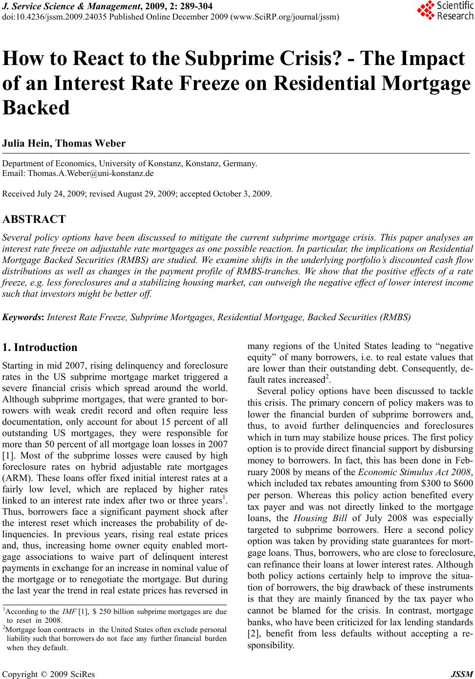