Journal of Applied Mathematics and Physics
Vol.07 No.08(2019), Article ID:94245,17 pages
10.4236/jamp.2019.78113
Numerical Simulations of Cavitation Flows around Clark-Y Hydrofoil
Yijie Liu, Jianhua Wang, Decheng Wan*
State Key Laboratory of Ocean Engineering, School of Naval Architecture, Ocean and Civil Engineering, Shanghai Jiao Tong University, Collaborative Innovation Center for Advanced Ship and Deep-Sea Exploration, Shanghai, China


Received: June 12, 2019; Accepted: August 9, 2019; Published: August 12, 2019
ABSTRACT
Cavitation is a complex flow phenomenon including unsteady characteristics, turbulence, gas-liquid two-phase flow. This paper provides a numerical investigation on comparing the simulation performance of three different models in OpenFOAM-Merkle model, Kunz model and Schnerr-Sauer model, which is helpful for understanding the cavitation flow. Considering the influence of vapor-liquid mixing density on turbulent viscous coefficient, the modified SST k-ω model is adopted in this paper to increase the computing reliability. The InterPhaseChangeFoam solver is utilized to simulate the two-dimensional cavitation flow of the Clark-Y hydrofoil with three cavitation models. The hydrodynamic performance including lift coefficient, drag coefficient and cavitation flow shape of the hydrofoil is analyzed. Through the comparison of the numerical results and experimental data, it is found that the Schnerr-Sauer model can get the most accurate results among the three models. And from the simulation point of water and water vapor mixing, the Merkle model has the best water and water vapor mixing simulation.
Keywords:
Cavitation Flow, OpenFOAM, Modified SST k-ω Model, Clark-Y Hydrofoil

1. Introduction
When the local pressure of flow field decreases below the saturated vapor pressure, explosive vaporization of liquid medium will occur, which is called cavitation. Cavitation is a complex flow phenomenon including unsteady characteristics, turbulence, gas-liquid two-phase flow. Due to the unsteady characteristics of the cavitation bubble, the pressure fluctuation during the collapse stage of the cavitation bubble will cause noise and vibration. According to the form of cavitation, the cavitation can be divided into sheet cavitation, vortex cavitation, cloud cavitation and bubble cavitation. Except for sheet cavitation, other types of cavitation have strong unsteady characteristics. Cavitation is inevitable on the mechanical surfaces of high-speed fluids such as hydrofoils and propellers which lead to blade erosion damage, accompanied by noise, vibration and other adverse effects. Therefore, more and more attention has been paid to the study of cavitation phenomena and unsteady characteristics of cavitation flows, both experimentally and numerically.
Early researchers [1] [2] have done a lot of model tests on hydrofoils to study the cavitation phenomenon. Kjeldsen et al. [3] performed cavitation observation using a 2D NACA0015 hydrofoil installed in a specially designed water tunnel. The results show that the characteristics of cavitation flows are affected by the angle of attack and cavitation number. Kawanami et al. [4] observed cloud cavitation on hydrofoil profiles using high-speed video and high-speed photographs and studied the mechanism of cloud cavitation on hydrofoil profile. Franc and Michel [5] studied the cavities formed through two-dimensional hydrofoils by measuring average and dynamic pressures, and further elaborated the cavitation physics. Fujii et al. [6] have further revealed the periodic behaviors of cavitation flow around hydrofoils through experiments. Amromin, E. et al. [7] designed an alternative hydrofoil by modifying the suction side of the traditional NACA0015 hydrofoil, providing a stable drag reduction through partial cavitation. Foeth et al. [8] [9] used time-resolved PIV method to design hydrofoil into a three-dimensional cavitation pattern closely related to propeller cavitation, and studied its effects on vibration, corrosion and noise.
Model experiment is of great importance for cavitation research. However, the high cost, severe scale effect and long period of the above model tests restrict our further research on cavitation problems. The development of numerical methods and computer processors has prompted researchers to further explore and study cavitation problems through numerical simulation. Potential flow simulation was used in the early stage [10] [11]. Due to the neglect of viscous effect, potential flow method is difficult and ineffective in dealing with three-dimensional problems. Therefore, viscous flow method has been widely used since the end of last century. At the same time, the research on cavitation of complex models such as propeller has also made remarkable progress. Chang et al. [12] analyzed the image results of cavitation generated by a propeller suction surface and evaluated the accuracy of the associated RANS (Reynolds-averaged Navier-Stokes) simulations. Hasuike et al. [13] studied the application of CFD in the transition flow and cavitation flow of marine propeller. Noble [14] used theoretical and numerical methods to predict the periodic back sheet cavitation on marine propellers operating in a ship’s wake. Peters et al. [15] used an implicit RANS-based flow solver and volume fluid method (VOF) to simulate the cavitation flow around a marine propeller. In addition to the numerical simulation of propeller, more efforts [16] are made to improve the main methods of viscous flow numerical simulation. Bensow [17] and others used RANS, DES (Direct Numerical Simulation) and LES (Large Eddy Simulation) methods to study the unsteady cavitation of Delft Twist 11 airfoil.
At present, the single-phase homogeneous model is mainly used to deal with the problem of cavitation flow. According to different definitions of the density field of y, the cavitation model can be classified into two types: one is based on the state equation and the other is based on the transport equation. Based on the equation of state, the density of a single medium is assumed to be a single-valued function of pressure, and the conversion between vapor and liquid is controlled by a function of density and pressure. Isentropic vaporization model, isothermal model and Rayleigh-Preset model represent three major branches. Shin [18] used the homogeneous equilibrium model to study the initiation and development of voids in vertical plates and elbows. It was found that with the decrease of void number, the resistance of vertical plates decreases, and the voids behind the plates will induce the formulation of super-cavitations. Based on the transport equation, the source term representing the vaporization and condensation process is used to simulate the mass transfer between vapor and water. The Singhal [19] model is based on the theory of bubble dynamics and derived from Rayleigh-Plesset equation [20]. Many factors affecting phase transition, such as bubble formation and pressure turbulence, are taken into account. Schnerr-Sauer model [21] is slightly different from Singhal model in giving the microscopic definition of volume fraction of gas phase. In Kunz [22] [23] model, the condensation rate is simplified by Ginzburg-Landau potential. Reboud et al. [24] revised the turbulent viscosity of k-epsilon model considering the local compressibility of the vapor-liquid mixing region. Based on these models, researchers [25] [26] have carried out extensive research on cavitation flow around hydrofoils.
This paper mainly simulates the hydrodynamic characteristics of the two-dimensional Clark-Y hydrofoils by using the interPhaseChangeFoam solver under the OpenFOAM platform. The lift coefficient, drag coefficient and cavitation flow of the hydrofoil are analyzed. The SST k-omega turbulence model is utilized, and the eddy viscosity coefficient of the turbulence model is modified to restrict the viscosity of the water vapor mixing zone. The simulation performance in two-dimensional cavitation flow of the Merkle model, Kunz model and Schnerr-Sauer model are also carried out. The structure of this paper is organized as follows: Section 1 presents the specific numerical simulation methods adopted in this study; in Section 2, the computational model for analysis is described and the results are discussed in Section 3; finally, several concluding remarks are made in Section 4.
2. Numerical Simulation Method
2.1. Governing Equations
Cavitation flow belongs to two-phase flow and there is continuous mass transformation between vapor phase and liquid phase in the two-phase flow. In order to solve a cavitation flow problem, the following equations need to be solved: continuity Equation (7), phase Equations (2) and (3) and momentum Equation (8). Before solving the problem, the volume fraction is define
(1)
In the cavitation flow, the continuity equation of each phase is given as:
(2)
(3)
In the above equations, l denotes liquid phase, V denotes vapor phase, is their volume fraction, is their density, U is their velocity vector, is the mass exchange between two phases. In the process of solution, only one phase equation needs to be solved because of the relationship between gas phase and liquid phase.
(4)
For the mixed medium consisting of vapor and liquid phases, it is satisfied that:
(5)
(6)
Among them, u is the velocity of mixed medium and ρ is the density of mixed medium.
The continuity equations for the simulation of cavitation flow are obtained:
(7)
According to the assumption of single-phase homogeneity, the momentum equation of vapor-liquid two-phase matter can be obtained:
(8)
The density and viscosity coefficients of mixed media are defined as follows:
(9)
(10)
2.2. Cavitation Models
In this paper, three cavitation models based on transport equation are used.
2.2.1. Merkle Model
The Merkle cavitation model is based on a vapor-liquid two-phase flow model, which derives the interphase mass transfer rate from the mixed density. The formula is:
(11)
(12)
In the Merkle model, is the reference speed; is the reference time. and are empirical coefficients, which are and , respectively.
and are expressions of mass exchange during vaporization and condensation, respectively.
2.2.2. Kunz Model
Kunz modified the Merkle model and simplified the Ginzburg-Landau potential for the condensation rate. It can be seen that the final condensation rate is proportional to the volume fraction of vapor, while the evaporation rate is proportional to the volume fraction of liquid phase and the difference of vapor-hydraulic pressure.
(13)
(14)
In the formula of the Kunz model, is the free-flow velocity; is the characteristic time scale, where L is the feature length; and are empirical constants. Generally, is the evaporation coefficient, and is the condensation coefficient. The appropriate value should be selected according to the specific model. The general value range is .
For the two empirical coefficients in the above formula, there is no uniform reference value, so different empirical coefficients need to be taken in different situations. Kunz model is considered to have the following characteristics: for sheet cavitation, the force at the vapor-liquid interface is more balanced, the pressure and velocity change range is small; it can deal with the high density ratio of cavitation flow, and the dependence on empirical constants is relatively high.
2.2.3. Schnerr-Sauer Model
The Schnerr-Sauer model is derived from Rayleigh-Plesset equation based on bubble dynamics theory. In Schnerr-Sauer model, the vapor volume fraction is expressed as follows:
(15)
In practical applications, considering the phase change is divided into two types, liquefaction and evaporation. The Schnerr-Sauer model equation is deduced:
(16)
(17)
The bubble radius R satisfies the following Formula (18), and can be obtained by the deformation of the Formula (15). and are the condensation and vaporization coefficients respectively. The Schnerr-Sauer model has proved to be a relatively reliable model after a large number of practical applications and verification. The researchers roughly summarize the following characteristics: It can be applied to mixed flows with a large number of spheres. In the case of cavitation; the expression of condensation rate and vaporization rate is symmetrical; it is used more frequently in cavitation flow around an approximate cylinder or sphere, which can better simulate the retroreflection flow.
(18)
2.2.4. SST k-Omega Turbulence Model and SST k-Omega Modified Turbulence Model
In SST k-omega model, k-omega model is used near the wall and k-epsilon model is used in the far field. At present, it is one of the widely used turbulence model, which can effectively avoid the problem that the k-omega model is too sensitive to the size of the entrance turbulence. Since the RANS turbulence model is developed on the basis of a single-phase and completely incompressible medium, the turbulent viscosity at the end of the cavitation will be over-predicted when the RANS model is used to simulate the cavitation flow.
Reboud et al. [27] modified the turbulent viscosity of the k-omega model considering the local compressibility of the vapor-liquid mixing region. This model assumes that a reduced, non-linear turbulent viscosity is added to the multiphase medium.
With the help of Reboud’s idea, this paper modifies the SST k-Omega model:
(19)
(20)
where k is turbulent energy, ω is turbulent dissipation rate, are constant, and ρ is fluid density. When the water vapor content is the same, after introducing the density function, especially in the vapor-liquid mixing region with high water vapor content, the influence of the over-predicted viscosity on the cavitation flow can be reduced, which can limit the excessive turbulence of the water vapor mixing zone in the cavitation tail, to simulate the Re-entrant and cavitation shedding more precisely. The parameter n in the modified turbulence model should be greater than 1, and some scholars recommend a value of not less than 10. After research [28], for the lift coefficient, the data obtained when n = 10 is more stable, and is closer to the experimental value. Therefore, it is considered that n = 10 is appropriate for the subsequent simulations.
3. Case Description of Clark-Y Hydrofoil
3.1. Computational Model
The 2D computational domain is shown in Figure 1. The size of the domain is 500 × 300 mm. And a chord length is extended in front of the leading edge of the domain and three chord lengths are extended behind the trailing edge. The test geometry is a Clark-Y hydrofoil at 8 degree angle of attack with chord length C = 100 mm.
3.2. Computational Grid
A region-wide background grid region is created firstly, then encrypted in the OpenFOAM via the snappy HexMesh method. This process is for better prediction of the forces on the Clark-Y two-dimensional hydrofoil and the cavitation on the suction surface of the blade. A sketch of the grid in the computational domain is shown in Figure 2. There are three parts in the grid system. The first
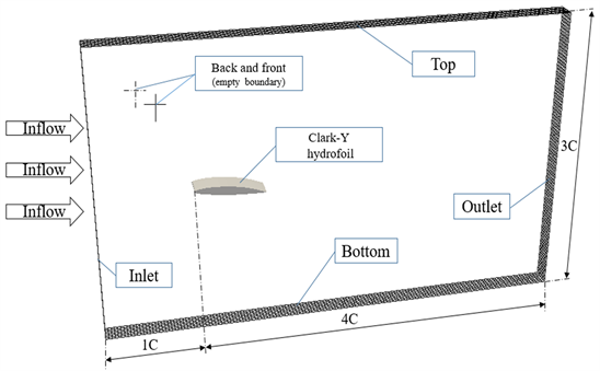
Figure 1. Computation domain.

Figure 2. Computational mesh around Clark-Y hydrofoil.
part is the outer net, which is the initial mesh of the entire flow field; the length is twice the length of the chord, and the height is 2D. Figure 2 is a refined mesh with three levels of refinement. The mesh in the entire computational domain grid is used for the simulation of the SST k-omega turbulence model and the improved SST k-omega turbulence model with a grid size of around 600,000 cells, with a computational time step of 0.0004 s.
3.3. Boundary Condition
The variables are initialized as follows:
Velocity U: The entrance is a fixed value U = 10 m/s, and the exit is a zero gradient. Pressure p: Reference pressure is obtained by the cavitation number through Equation (21). The cavitation number in the present work is 0.8.
(21)
4. Results and Discussion
4.1. Analysis of Two-Dimensional Hydrofoil Cavitation Flow Simulation
The surface of the hydrofoil can form a layer of cavitation. In this paper, three models are used to simulate the cavitation flow of two-dimensional hydrofoil Clark-Y. The cavitation clouds of Clark-Y hydrofoil computed by three different models are shown in the following figures, from Figures 3-5. As can be seen from the figures, a thin layer of cavitation generally appears on the surface of hydrofoil and grows from the front of hydrofoil. This layer of cavitation is close to the surface of hydrofoil, also known as sheet cavitation. Sheet cavitation is one of the main cavitation forms of hydrofoil.

Figure 3. Simulation of cavitation with Merkle model.

Figure 4. Simulation of cavitation with Kunz model.

Figure 5. Simulation of cavitation with Schnerr-Sauer model.
The cyclic variation of the cavitation flow in a period of the numerical simulation can be summarized according to the simulation results:
1) A sheet-like cavitation zone is formed from the front of the hydrofoil to the surface like the cavitation zone in Figure 5(a). When the upstream flow collides with the front of the hydrofoil, flow separation occurs and a low pressure zone is formed on the surface. The pressure in the low pressure zone is lower than the saturated vapor pressure of water at this temperature, which leads to a large amount of vaporization of water. The vaporization of water leads to the formation of cavitation.
2) The sheet cavitation zone grows correspondingly. When the upstream flow flows to the rear, the low-pressure zone becomes longer and longer. The sheet cavitation zone can be seen from Figure 4(a) to Figure 5(b).
3) Cavitation zone begins to break and then shed. Because the sheet cannot continue to grow after the cavitation grows to a certain extent. Then the cavitation zone will shed, which is caused by the re-entrant jet. The shedding phenomena in the cavitation zone can be seen from Figure 3(e), Figure 3(f) and Figure 5(c).The fracture phenomena in the cavitation zone can be seen from Figure 3(b) to Figure 3(c).
4) Formation of cloud cavitation. The falling cavitation forms cloud-like cavitation under the shear action of upstream inflow and return jet, and moves downstream. At the same time, the next period of sheet cavitation begins at the front of hydrofoil. The formation of cloud cavitation can be found from Figure 5(e) to Figure 5(f).
From the simulation point of water and water vapor mixing, the Merkle model has the best water and water vapor mixing simulation and is more accurate than the Schnerr-Sauer model. The effect of the Kunz model in simulating water vapor mixing is very general. In the cavitation cloud diagram of Figure 3, there is a significant mixing process between the gas phase and the liquid phase. This result is related to the equation of the Merkle model, which is based on a vapor-liquid two-phase flow model, which derives the interphase mass transfer rate from the mixed density. Therefore, compared with the other two models, the Merkle model can achieve a good simulation of water vapor mixing.
Compared with the cavitation flow diagrams of model tests (Figure 6), the variation of cavitation flow in numerical simulation is accurate. A complete cycle can be summarized as growth, truncation, shedding, cloud cavitation and re-formation of sheet cavitation. There are obvious differences in the simulation of hydrofoil cavitation flow under different cavitation models. The simulation of

Figure 6. Experimental results.
cavitation flow in Merkle model shows a complete cavitation period. From Figure 3(b) to Figure 3(c), it can be seen that the growth of cavitation flow will fracture when it comes to a certain extent. However, the simulation of truncation and shedding process is not particularly precise, and the cavitation fragments are large. The simulation of cavitation flow in Kunz model is quite different from the other two models, and the cavitation zone at the front of hydrofoil has hardly changed during the whole period. The growth, truncation and shedding of partial cavitation flow will occur in the cavitation zone at the tail of the hydrofoil. However, it is not suitable to simulate the whole cavitation flow of the Clark-Y hydrofoil. In the Schnerr-Sauer model, many evident cavitation shedding can be observed, which is a continuous process from the growth of cavitation to truncation and then to shedding. And the size of the fragments falling off in the Schnerr-Sauer model can be captured effectively. Many details in the simulation of cavitation flow are presented. From the point of view of the cavitation cloud, the simulation results obtained by using Schnerr-Sauer model can accurately describe the variation law of cavitation.
4.2. Analysis and Comparison of Hydrodynamic Characteristics of Different Models
The time history curve of lift and drag coefficients of two-dimensional hydrofoils calculated by three models are shown in Figure 7-9. The results of lift and drag coefficients of different models and other researchers’ work are listed in Table 1. From Figures 7-9, the shapes of time history curves of lift and drag coefficients of the three models are approximately similar. Comparing to Zhao’s research [29] about cavitation around Clark-Y, the simulation method is credible. The time history curves in Figure 7 are relatively flat, with only 2 - 3 fluctuations in a cycle. The shapes of the curves in Figure 7 are also consistent with the phenomenon in Figure 4. The ability of Kunz model to simulate the generation and growth of cavitation is gentle, and it is difficult to see the splitting and shedding of cavitation in the whole process. Therefore, it is difficult to see the fluctuation of the curve in Figure 7. In Figure 8 the time history curves have a lot of fluctuations compared with the curves in Figure 7. The change of the time history curve in Figure 9 corresponds to the variation period of cavitation in Figure 3. A complete cavitation cycle can be observed in Figure 3. Thus, the periodic fluctuation characteristics of the time history curves are obvious in Figure 8. That is to say, Merkle model can simulate the generation, growth and shedding of cavitation accurately. The time history curves in Figure 9 clearly have the most obvious fluctuations. The large number of violent fluctuations in Figure 9 indicates that Schnerr-Sauer model can accurately capture many small bubble generated during the cavitation process. These violent fluctuations also correspond to the small vacuoles observed in Figure 9. Obviously, there are abundant details in the simulation of the cavitation flow field under the Schnerr-Sauer model. Compared with other researchers’ work listed in Table 1, the lift and drag coefficients of three different models are accurate. And the
 (a)
(a)
 (b)
(b)
Figure 7. Time history curve of lift and drag coefficients of Kunz model. (a) Variation of lift coefficient with time; (b) Variation of drag coefficient with time.
 (a)
(a)
 (b)
(b)
Figure 8. Time history curve of lift and drag coefficients of Merkle model. (a) Variation of lift coefficient with time; (b) Variation of drag coefficient with time.
 (a)
(a)
 (b)
(b)
Figure 9. Time history curve of lift and drag coefficients of Schnerr-Sauer model. (a) Variation of lift coefficient with time; (b) Variation of drag coefficient with time.

Table 1. Quantities measured by experiment and predicted by the different turbulence models.
result of Schnerr-Sauer model is more accurate than the results of Kunz model and Merkle model.
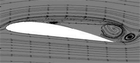
4.3. Analysis of the Cause for Cavitation Shedding
The figures for cavitation simulation in Schnerr-Sauer model is close to the experimental cavitation image. The phenomenon of cavitation in Schnerr-Sauer model fracture and shedding with time is more obvious which is in good agreement with the experimental results. And Schnerr-Sauer model can capture abundant small vortices accurately. The velocity vector diagram during cavitation shedding is shown in Figure 10. The distribution of speed when cavitation shedding is shown in Figure 11. Analyzing these figures, it can be found that the retraction at the junction between the end of the inner cavity and the hydrofoil indicates that there is a re-entrant jet, which causes the small bubbles to fall off at the end of the inner cavity. Due to the different velocities of flow on the upper and lower surfaces of hydrofoils, a clockwise rotating vortex structure is formed at the tail end when the flow reaches the tail of hydrofoils. The existence of re-entrant and vortex structure can be found in Figure 10. Vortex structure leads to re-incident flow, and cloud cavitation is caused by shear during collision. Hence the vortex and re-entrant jet is the main cause of cavitation shedding. Both of images in Figure 11(a) and Figure 11(b) showed the existence of the re-entrant. In Figure 10(c) the existence of re-entrant can be found.
5. Conclusion
In this paper, a numerical investigation on comparing the simulation performance of three different models in OpenFOAM-Merkle model, Kunz model and Schnerr-Sauer model is provided. The SST k-omega model is modified and the modified SST k-omega model can better reflect the initial, development and collapse of the vacuole, so as to better study the cavitation problem. The latter SST k-omega model is a more accurate turbulence model for predicting cavitation. And three different cavitation models Kunz, Merkle and Schnerr-Sauer are used to simulate the cavitation around Clark-Y hydrofoil by using interPhaseChangeFoam solver in OpenFOAM. The Merkle model has the best water and water vapor mixing simulation and is more accurate than the Schnerr-Sauer
 (a)
(a) (b)
(b) (c)
(c)
Figure 10. Velocity vector of the flow fields. (a) Streamline diagram; (b) Streamline diagram; (c) Re-entrant jets.
 (a)
(a) (b)
(b) (c)
(c)
Figure 11. Velocity field of hydrofoil during cavitation shedding. (a) Numerical result; (b) Numerical result; (c) Experimental result.
model. The hydrodynamic characteristics are demonstrated and compared. Merkle model and Schnerr-Sauer model are better than Kunz model in simulating unsteady cavitation flow, which are in good agreement with the experimental results, and the unsteady characteristics of cavitation change periodically. Compared with model Merkle, model Schnerr-Sauer can capture abundant small vortices and simulate unsteady cavitation flow around two-dimensional hydrofoils more accurately. The hydrodynamic performance including lift coefficient, drag coefficient and cavitation flow shape of the hydrofoil is analyzed. With Schnerr-Sauer model, a more accurate simulation result is achieved. Further research on re-entry jet shows that the vortex structure at the tail of hydrofoil is the main cause of cavitation shedding. In the follow-up study, the Schnerr-Sauer model can be used to further study the hydrodynamic characteristics of E779A propeller under the wake flow field.
Acknowledgements
This work is supported by the National Natural Science Foundation of China (51879159, 51490675, 11432009, 51579145), Chang Jiang Scholars Program (T2014099), Shanghai Excellent Academic Leaders Program (17XD1402300), Program for Professor of Special Appointment (Eastern Scholar) at Shanghai Institutions of Higher Learning (2013022), Innovative Special Project of Numerical Tank of Ministry of Industry and Information Technology of China (2016-23/09) and Lloyd’s Register Foundation for doctoral student, to which the authors are most grateful.
Conflicts of Interest
The authors declare no conflicts of interest regarding the publication of this paper.
Cite this paper
Liu, Y.J., Wang, J.H. and Wan, D.C. (2019) Numerical Simulations of Cavitation Flows around Clark-Y Hydrofoil. Journal of Applied Mathematics and Physics, 7, 1660-1676. https://doi.org/10.4236/jamp.2019.78113
References
- 1. Kawakami, D.T., Fujii, A., Tsujimoto, Y. and Arndt, R.E.A. (2008) An Assessment of the Influence of Environmental Factors on Cavitation Instabilities. Fluids Eng, 130. https://doi.org/10.1115/1.2842146
- 2. Laberteaux, K.R. and Ceccio, S.L. (2001) Partial Cavity Flows. Part 2. Cavities Forming on Test Objects with Spanwise Variation. Journal of Fluid Mechanics, 431, 43-63. https://doi.org/10.1017/S0022112000002937
- 3. Kjeldsen, M. (2000) Spectral Characteristics of Sheet and Cloud Cavitation. Journal of Fluids Engineering, 122, 481-487. https://doi.org/10.1115/1.1287854
- 4. Kawanami, Y., Kato, H., Yamaguchi, H., Tanimura, M. and Tagaya, Y. (1997) Mechanism and Control of Cloud Cavitation. Fluids Eng, 119, 788-794. https://doi.org/10.1115/1.2819499
- 5. Franc, J.P. and Michel, J.M. (2004) Michel Fundamentals of Cavitation. Kluwer Academic Publishers.
- 6. Fujii, D.T., Kawakami, Y., Tsujimoto and Arndt, R.E.A. (2007) Effect of Hydrofoil Shape on Cavity Oscillation. Fluids Eng, 129, 669-674. https://doi.org/10.1115/1.2734183
- 7. Amromin, E., Kopriva, J., Arndt, R.E.A. and Wosnik, M. Hydrofoil Drag Reduction by Partial Cavitation. Journal of Fluids Engineering, 128, 931-936. https://doi.org/10.1115/1.2234787
- 8. Foeth, E.J., van Doorne, C.W.H., van Terwisga, T. and Wieneke, B. (2006) Time Resolved PIV and Flow Visualization of 3D Sheet Cavitation. Exp. Fluids, 40, 503-513. https://doi.org/10.1007/s00348-005-0082-9
- 9. Foeth, E.J., van Terwisga, T. and van Doorne, C. (2008) On the Collapse Structure of an Attached Cavity on a Three-Dimensional Hydrofoil. Fluids Eng, 130, Article ID: 071303. https://doi.org/10.1007/s00348-005-0082-9
- 10. Kinnas, S.A. and Fine, E. (1993) A Numerical Nonlinear Analysis of the Flow around 3-D Cavitating Hydrofoil. Journal of Fluid Mechanics, 254, 151-181. https://doi.org/10.1017/S0022112093002071
- 11. Tulin, M.P. (2010) Steady Two-Dimensional Cavity Flows about Slender Bodies. IEEE Transactions on Magnetics, 4707-4709.
- 12. Chang, Y.C., Hu, C.N. and Tu, J.C. (2010) Experimental Investigation and Numerical Prediction of Cavitation Incurred on Propeller Surfaces. Journal of Hydrodynamics, 22, 764-769. https://doi.org/10.1016/S1001-6058(10)60028-5
- 13. Hasuike, N., Yamasaki, S. and Ando, J. (2011) Numerical and Experimental Investigation into Propulsion and Cavitation Performance of Marine Propeller.4th International Conference on Computational Methods in Marine Engineering.
- 14. Noble, D.J. (1987) Numerical Prediction of Unsteady Sheet Cavitation on Marine Propel-lers.
- 15. Peters, A., Lantermann, U. and Moctar, O.E. (2018) Numerical Prediction of Cavitation Erosion on a Ship Propeller in Model- and Full-Scale. Wear, S0043164817316307. https://doi.org/10.1016/j.wear.2018.04.012
- 16. Kim, S.E. (2009) A Numerical Study of Unsteady Cavitation on a Hydrofoil. Proceedings of the 7th International Symposium on Cavitation.
- 17. Bensow, R. (2011) Simulation of the Unsteady Cavitation on the Delft Twist11 Foil Using RANS, DES and LES. International Symposium on Marine Propulsors Workshop Proceedings.
- 18. Hejranfar, K. and Ezzatneshan, E. (2009) A Dual-Time Implicit Preconditioned Navier-Stokes Method for Solving 2D Steady/Unsteady Laminar Cavitating/Noncavitating Flows Using a Barotropic Model.
- 19. Singhal, A.K., Mahesh, M.A. and Lu, H.Y. (2002) Mathematical Basis and Validation of the Full Cavitation Model. Journal of Fluids Engineering, 124, 617-624. https://doi.org/10.1115/1.1486223
- 20. Brennen, C.E. (1995) Cavitation and Bubble Dynamics. Oxford University Press.
- 21. Schnerr, G.H. and Sauer, J. (2001) Physical and Numerical Modeling of Unsteady Cavitation Dynamics. 4th International Conference on Multiphase Flow.
- 22. Merkle, C.L., Feng, J. and Buelow, P.E. (1998) Computational Modeling of the Dynamics of Sheet Cavitation. 3th International Symposium on Cavitation.
- 23. Medvitz, R.B., Kunz, R.F. and Boger, D.A. (2002) Performance Analysis of Cavitating Flow in Centrifugal Pumps Using Multiphase CFD. Journal of Fluids Engineering, 124, 377-383. https://doi.org/10.1115/1.1457453
- 24. Reboud, J.L., Stutz, B. and Coutier-Delgosha, O. (1998) Two Phase Flow Structure of Cavitation Experiment and Modeling of Unsteady Effects. 3rd Int. Sym. Cavitation.
- 25. Lu, N.-X., Bensow, R.E. and Bark, G. (2010) LES of Unsteady Cavitation on the Delft Twisted Foil. Journal of Hydrodynamics, 22, 784-791. https://doi.org/10.1016/S1001-6058(10)60031-5
- 26. Karabelas, S.J., Koumroglou, B.C. and Argyropoulos, C.D. (2012) High Reynolds Number Turbulent Flow Past a Rotating Cylinder. Applied Mathematical Modelling, 36, 379-398. https://doi.org/10.1016/j.apm.2011.07.032
- 27. Coutierdelghosa, O., Patella, R.F. and Reboud, J.L. (2003) Evaluation of the Turbulence Model Influence on the Numerical Simulation of Unsteady Cavitation. Journal of Fluids Engineering, 125, 38-45. https://doi.org/10.1115/1.1524584
- 28. Li, Y., Chen, K. and Wan, D. (2018) Numerical Study of Cavitation Shedding around NACA66 Hydrofoil Based on OpenFOAM. CCCM-ISCM.
- 29. Zhao, M. and Wan, D. (2018) Numerical Investigation of Cloud Cavitation Flows around Clark-Y Hydrofoil. 3rd International Symposium of Cavitation and Multiphase Flow.