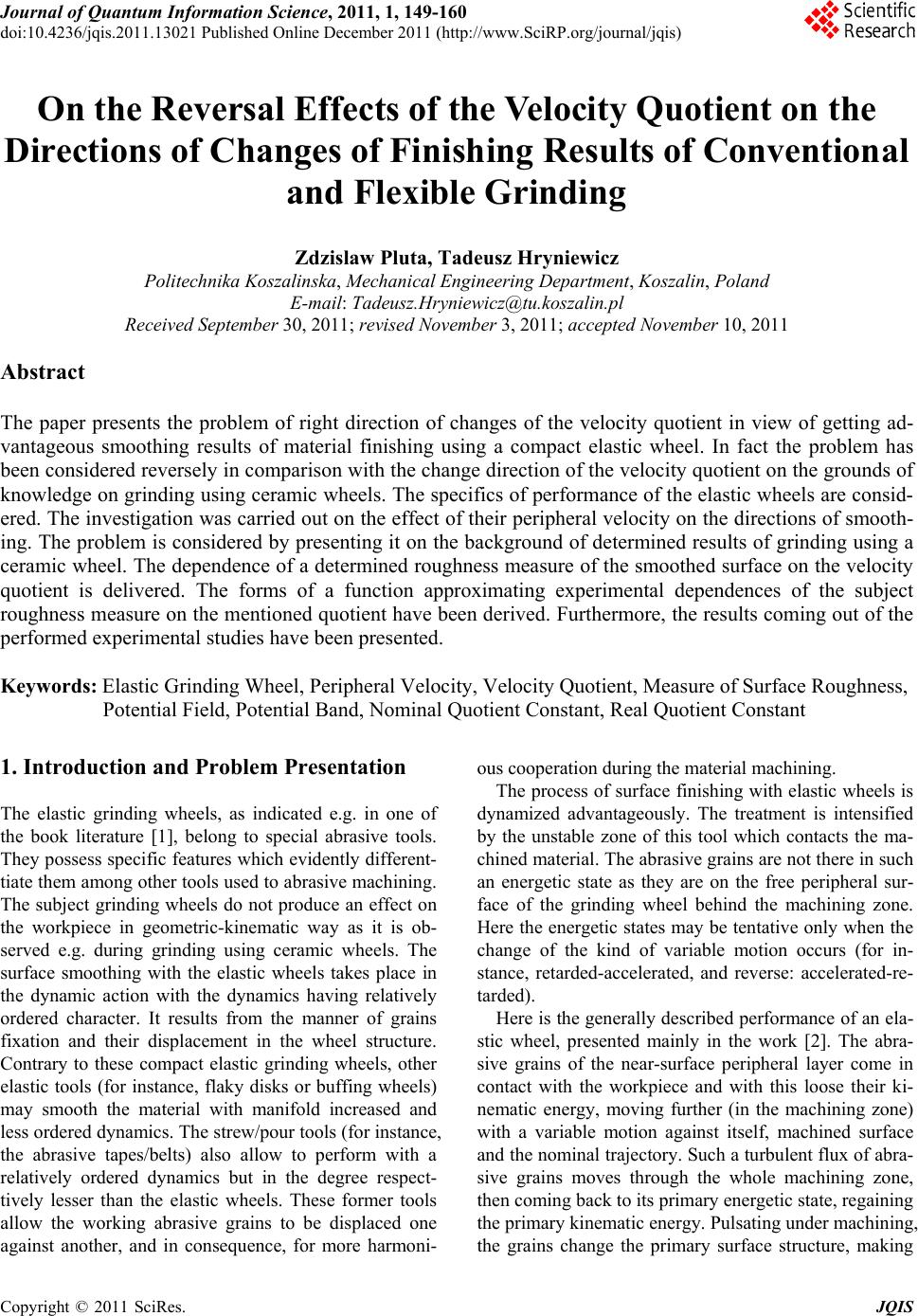
Journal of Quantum Informatio n Science, 2011, 1, 149-160
doi:10.4236/jqis.2011.13021 Published Online December 2011 (http://www.SciRP.org/journal/jqis)
149
On the Reversal Effects of the Velocity Quotient on the
Directions of Changes of Finishing Results of Conventional
and Flexible Grinding
Zdzislaw Pluta, Tadeusz Hryniewicz
Politechnika Koszalinska, Mechanical Engineering Department, Koszalin, Poland
Received September 30, 2011; revised November 3, 2011; accepted November 10, 2011
Abstract
The paper presents the problem of right direction of changes of the velocity quotient in view of getting ad-
vantageous smoothing results of material finishing using a compact elastic wheel. In fact the problem has
been considered reversely in comparison with the change direction of the velocity quotient on the grounds of
knowledge on grinding using ceramic wheels. The specifics of performance of the elastic wheels are consid-
ered. The investigation was carried out on the effect of their peripheral velocity on the directions of smooth-
ing. The problem is considered by presenting it on the background of determined results of grinding using a
ceramic wheel. The dependence of a determined roughness measure of the smoothed surface on the velocity
quotient is delivered. The forms of a function approximating experimental dependences of the subject
roughness measure on the mentioned quotient have been derived. Furthermore, the results coming out of the
performed experimental studies have been presented.
Keywords: Elastic Grinding Wheel, Peripheral Velocity, Velocity Quotient, Measure of Surface Roughness,
Potential Field, Potential Band, Nominal Quotient Constant, Real Quotient Constant
1. Introduction and Problem Presentation
The elastic grinding wheels, as indicated e.g. in one of
the book literature [1], belong to special abrasive tools.
They possess specific features which evidently different-
tiate them among other tools used to abrasive machining.
The subject grinding wheels do not produce an effect on
the workpiece in geometric-kinematic way as it is ob-
served e.g. during grinding using ceramic wheels. The
surface smoothing with the elastic wheels takes place in
the dynamic action with the dynamics having relatively
ordered character. It results from the manner of grains
fixation and their displacement in the wheel structure.
Contrary to these compact elastic grinding wheels, other
elastic tools (for instance, flaky disks or buffing wheels)
may smooth the material with manifold increased and
less ordered dynamics. The strew/pour tools (for instance,
the abrasive tapes/belts) also allow to perform with a
relatively ordered dynamics but in the degree respect-
tively lesser than the elastic wheels. These former tools
allow the working abrasive grains to be displaced one
against another, and in consequence, for more harmoni-
ous cooperation during the material machining.
The process of surface finishing with elastic wheels is
dynamized advantageously. The treatment is intensified
by the unstable zone of this tool which contacts the ma-
chined material. The abrasive grains are not there in such
an energetic state as they are on the free peripheral sur-
face of the grinding wheel behind the machining zone.
Here the energetic states may be tentative only when the
change of the kind of variable motion occurs (for in-
stance, retarded-accelerated, and reverse: accelerated-re-
tarded).
Here is the generally described performance of an ela-
stic wheel, presented mainly in the work [2]. The abra-
sive grains of the near-surface peripheral layer come in
contact with the workpiece and with this loose their ki-
nematic energy, moving further (in the machining zone)
with a variable motion against itself, machined surface
and the nominal trajectory. Such a turbulent flux of abra-
sive grains moves through the whole machining zone,
then coming back to its primary energetic state, regaining
the primary kinematic energy. Pulsating under machining,
the grains change the primary surface structure, making

Z. PLUTA & T. HRYNIEWICZ
150
it more advantageous from the viewpoint of expected
technological requirements. The claims of improvement
of the surface roughness and the growth of gloss of sur-
face are the most important.
In contact with the machined workpiece the abrasive
grains decrease their inertia and centrifugal reaction
whereas the elasticity of their fixations may change not
only quantitatively, but also qualitatively. The bond, first
extended, attempts to return to the zero state, and at the
greater in-feeds may even undergo the compression. The
grains in this zone perform the work which is non-be-
havioral, because their firm energetic states are not pre-
served.
That is the specifics of performance of the compact
elastic grinding wheels, manufactured by many compa-
nies of abrasive manufacture profile [3-8]. It would be
useful and advantageous to present the subject abrasive
tools in view of revealing some essential differences be-
tween the performance of elastic and rigid (ceramic)
grinding wheels. The reference to the ceramic wheel will
be still necessary. Of course, that provided the compara-
tive analysis is to be concerned on the influence of pe-
ripheral velocity on the determined machining effects.
To reveal the essential problem it is worthy comparing
the two totally different ways of abrasive machining:
grinding and finishing/smoothing, i.e. the machining of
material with a rigid wheel (usually ceramic), and a
compact elastic wheel. The technology of grinding using
a ceramic wheel is generally known. However, it is wor-
thy noting a comparative criterion that is the peripheral
velocity of wheel and its influence on the finishing re-
sults of the treatment which is the surface roughness.
It is known that with the increase of peripheral veloc-
ity of ceramic grinding wheel the roughness of the ma-
chined surface decreases, respectively; it has been pre-
sented in the literature [9-11]. It is connected, as ex-
plained in the work [12], with the decrease of thickness
of the layer cut by a single edge and the increasing
amount of heat in the machining zone, and with this the
temperature of elements of the machining system. The
work [13] adds that then the grains loading decreases,
and with this the grinding wheel performs as more hard.
The consequence of such a performance of the wheel is
longer work of its grains, which is less frequency of its
spalling. Together with the increase of peripheral veloc-
ity of the grinding wheel, as mentioned above, the fre-
quency of the grain contact with the machined material is
greater, whereas the time of this contact is lesser, res-
pecttively.
These advantageous conditions, favouring the de-
crease of roughness, are illustrated by a plot (Figure 1)
excerpted from the reference [12], being the image of the
dependence of the surface unevenness height (created by
Figure 1. Dependence of measures a
R
,
z
R
of surface
roughness (formed by a material grinding) on the velocity
quotient v and the peripheral velocity of grinding
wheel [12].
qs v
the material grinding) on the peripheral velocity of the
grinding wheel, that is

z
s
Rfv. The same curve
relates also with the dependence of arithmetic mean of
the profile deviation of the mean line, that is a, on the
velocity quotient v, so the ratio of the peripheral ve-
locity
R
q
s
v of the grinding wheel to the peripheral veloc-
ity
p
v of the ground workpiece. Concerning this, the
plot covers also the coordinates axes, related to the men-
tioned magnitudes.
The hardened manganese steel (C = 0.5%, Mn = 1%)
was used as a ground material. The tool was the grinding
wheel of the grain size No. 46 made of semi-precious
aloxite 97A. The peripheral velocity of the ground work-
piece was assumed
p
v = 30 m·min–1, and the longitu-
dinal feed 0.3 12
p
aH

 mm·rev–1, where H is the
width of the wheels. There were two values of depth e
of the grinding wheel penetration in the machined mate-
rial: 0.01 and 0.05 mm.
a
Of course, that range of variability of the peripheral
velocity of grinding wheel does not exhaust the kine-
matic possibilities of the wheel at all. Here the upper
limit of the variability interval of this parameter was
caused by the shattering effect of the wheel (its resis-
tance to disrupture). Under other conditions the wheels
rotate with the velocities
s
v equal: 100 m·s–1 [9], and
even 320 m·s–1 [10]. Furthermore, that kinematic pa-
rameter results from the given resistance criterion of the
tool with both of them being correlated positively: the
greater strength of the wheel to disrupture (shattering),
the higher its peripheral velocity.
Moreover, taking into account the finishing/smooth-
ness criterion one should note the wheel should operate

151 Z. PLUTA & T. HRYNIEWICZ
with the highest possible velocity. Here both the rough-
ness and the velocity are correlated negatively. That
means the increase in peripheral velocity of the wheel
results in the decrease of roughness of the newly created
surface. Thus, to obtain the advantageous surface results
the highest possible peripheral velocity should be pro-
vided to the grinding wheel. That is the so called the gold
rule of grinding.
The quest of connection of surface roughness with the
peripheral velocity of the grinding wheel (also the veloc-
ity quotient) is then determined univocally and used in
practice; however, the relations of these magnitudes re-
ferred to the compact elastic wheels have not been as-
sumed and/or used until now. Then it is worthy present-
ing first the history of usage of these grinding wheels,
together with the outline of their development and stu-
dies over the influence of the peripheral velocity of this
type of tools on the directions of changes of the finishing
results of smoothing.
To solve the problem, first the history of usage of the
compact elastic wheels and the effect of their peripheral
velocity on the directions of changes of the finishing
results of treatment, are delivered. Those special abrasive
tools, covering one of many manufactured geometric
assortments, are made in Poland by the Fabryka Tarcz
Ściernych in Grodzisk Mazowiecki [5]; their production
was begun in 1973. There were only some foreign com-
panies, such as SLIP-NAXOS [3], ARTIFEX [4],
KLINGSPOR [6], and LUKAS [7] which started to do it
earlier. These tools contain the abrasive grains displaced
in the entire mass of the resin bond, so they are compact
tools.
The work [14] treats on polishing using the single
crystals of silicon by the elastic aloxite grinding wheels.
The way of manufacture of that kind of wheels has been
also described. The process of their manufacture con-
sisted of the following stages: mixing the polyurethane
and abrasive grains; smearing the mixture over the steel
base plate creating the layer of thickness of about 15 mm;
leaving such prepared abrasive-polyurethane material for
3 - 4 days for the chemical reactions to occur. It is wor-
thy mentioning that the Polish literature [15,16] treats in
extension on the manufacture of the polyurethane elastic
abrasive tools.
The journal “Werkstatt und Betrieb” covers the results
of finishing of the steel SW18 and the brass MO59 by
means of elastic wheels of the properly differentiated
characteristics [17], as well as the results of cutting ma-
terials using flexibly fixed grains of the post-copper slag
[18]. “Schleifen und Trennen” presents some aspects of
manufacture and usage of the grinding wheels of porous
elastic wheels [19].
It is worthy turning the attention on the work [11],
published by the journal “Maschinen und Werkzeug”.
Based on the example of the grinding wheels of Artifex
the advantages of abrasive tools on the elastic bond (of
the flexibility detected even on touch), have been dis-
cussed. It was stated that the use of these wheels requires
the relative high rotational velocities especially in rela-
tion to the grinding pins (diameters of 5 to 30 mm). It is
treated about a high cutting output of which the per-
formance is achieved at not a big compression force and
the tool velocity, equaling up to 30 m·s–1.
On the world edition market the problems of finishing
using the compact elastic wheels has been noted only in
recent decade. At the beginning of this decade (2001) a
work appeared treating of the curvilinear finishing of
surfaces using the grinding pins of a special design [20].
The concept, structure, shape, and the manufacture pro-
cedure of the susceptible abrasive tool made of thermo-
setting polyurethane elastomer coated with abrasive ma-
terial of aluminum oxide, have been discussed there.
This tool enables the finishing treatment thanks to the
ability to deform and conforming the shape of the ma-
chined surface in the machining zone. The following
effects were studied, such as: obtained surface roughness,
the mentioned machining effectiveness and durability in
the process of treatment of high-alloy tool steel, previ-
ously machined by milling.
Then the work [21] appeared, concerned with elastic
properties of the flexible abrasive tools of polyurethane
bonds. There the results of the studies of the wheel prop-
erties with the outline of their modification in view of
increasing the effectiveness of the process of abrasive
smoothing have been presented.
Recently, in 2009, the works [22,23] appeared. The ar-
ticle [22] presents first the characteristics of the initial
conditions, relating to the peripheral smoothing using
elastic wheels. These conditions are determined by the
incision angle, depending on the peripheral velocity of
the grinding wheel, in-feed, and the workpiece velocity.
Such a determined dependence was used to forecast the
directions of roughness changes. It was stated, based on
the results of experimental verification of the prognoses,
that the finishing results of the peripheral smoothing may
be anticipated with a success, making use of the men-
tioned prognosis indicator.
The work [23] explains much wider those initial con-
ditions of cutting. It has been proved that one cannot
smooth a material using a rotating wheel with a critical
velocity, which the velocity is connected with the wheel
resistance to disrupture. The wheel velocity has to be
respectively lower, because in that case the effect of the
grain size on the surface roughness is significantly less,
and moreover it affects advantageously the finishing re-
sults of the smoothing.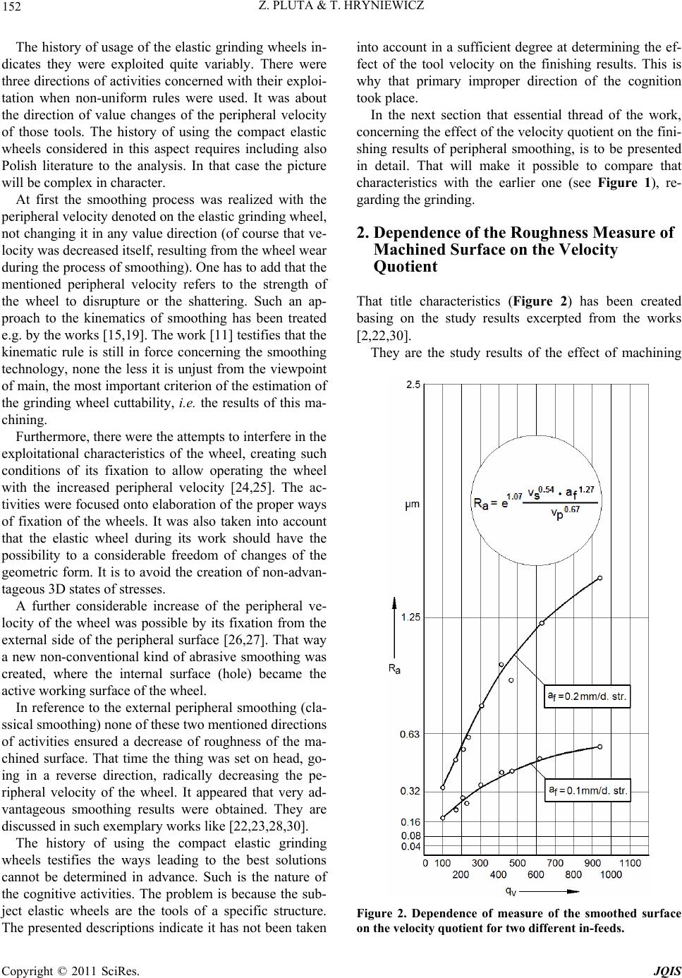

Z. PLUTA & T. HRYNIEWICZ
152
The history of usage of the elastic grinding wheels in-
dicates they were exploited quite variably. There were
three directions of activities concerned with their exploi-
tation when non-uniform rules were used. It was about
the direction of value changes of the peripheral velocity
of those tools. The history of using the compact elastic
wheels considered in this aspect requires including also
Polish literature to the analysis. In that case the picture
will be complex in character.
At first the smoothing process was realized with the
peripheral velocity denoted on the elastic grinding wheel,
not changing it in any value direction (of course that ve-
locity was decreased itself, resulting from the wheel wear
during the process of smoothing). One has to add that the
mentioned peripheral velocity refers to the strength of
the wheel to disrupture or the shattering. Such an ap-
proach to the kinematics of smoothing has been treated
e.g. by the works [15,19]. The work [11] testifies that the
kinematic rule is still in force concerning the smoothing
technology, none the less it is unjust from the viewpoint
of main, the most important criterion of the estimation of
the grinding wheel cuttability, i.e. the results of this ma-
chining.
Furthermore, there were the attempts to interfere in the
exploitational characteristics of the wheel, creating such
conditions of its fixation to allow operating the wheel
with the increased peripheral velocity [24,25]. The ac-
tivities were focused onto elaboration of the proper ways
of fixation of the wheels. It was also taken into account
that the elastic wheel during its work should have the
possibility to a considerable freedom of changes of the
geometric form. It is to avoid the creation of non-advan-
tageous 3D states of stresses.
A further considerable increase of the peripheral ve-
locity of the wheel was possible by its fixation from the
external side of the peripheral surface [26,27]. That way
a new non-conventional kind of abrasive smoothing was
created, where the internal surface (hole) became the
active working surface of the wheel.
In reference to the external peripheral smoothing (cla-
ssical smoothing) none of these two mentioned directions
of activities ensured a decrease of roughness of the ma-
chined surface. That time the thing was set on head, go-
ing in a reverse direction, radically decreasing the pe-
ripheral velocity of the wheel. It appeared that very ad-
vantageous smoothing results were obtained. They are
discussed in such exemplary works like [22,23,28,30].
The history of using the compact elastic grinding
wheels testifies the ways leading to the best solutions
cannot be determined in advance. Such is the nature of
the cognitive activities. The problem is because the sub-
ject elastic wheels are the tools of a specific structure.
The presented descriptions indicate it has not been taken
into account in a sufficient degree at determining the ef-
fect of the tool velocity on the finishing results. This is
why that primary improper direction of the cognition
took place.
In the next section that essential thread of the work,
concerning the effect of the velocity quotient on the fini-
shing results of peripheral smoothing, is to be presented
in detail. That will make it possible to compare that
characteristics with the earlier one (see Figure 1), re-
garding the grinding.
2. Dependence of the Roughness Measure of
Machined Surface on the Velocity
Quotient
That title characteristics (Figure 2) has been created
basing on the study results excerpted from the works
[2,22,30].
They are the study results of the effect of machining
Figure 2. Dependence of measure of the smoothed surface
on the velocity quotient for two different in-feeds.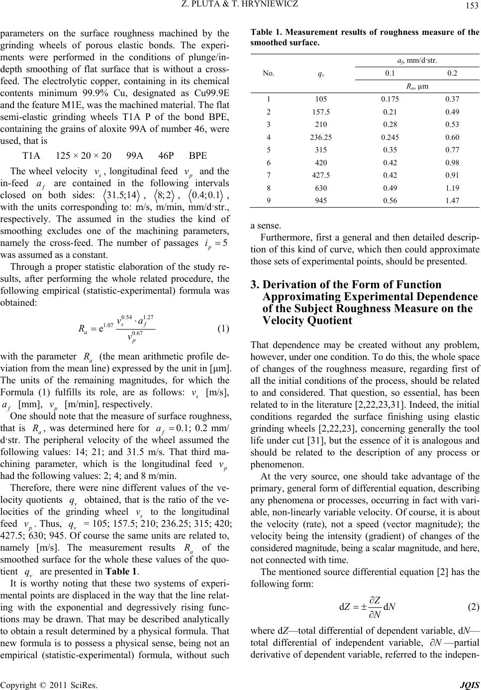

153 Z. PLUTA & T. HRYNIEWICZ
parameters on the surface roughness machined by the
grinding wheels of porous elastic bonds. The experi-
ments were performed in the conditions of plunge/in-
depth smoothing of flat surface that is without a cross-
feed. The electrolytic copper, containing in its chemical
contents minimum 99.9% Cu, designated as Cu99.9E
and the feature M1E, was the machined material. The flat
semi-elastic grinding wheels T1A P of the bond BPE,
containing the grains of aloxite 99A of number 46, were
used, that is
T1A 125 × 20 × 20 99A 46P BPE
The wheel velocity
s
v, longitudinal feed
p
v and the
in-feed
f
a are contained in the following intervals
closed on both sides: 31.5; , 14 8; 2, 0.4;0.1 ,
with the units corresponding to: m/s, m/min, mm/d·str.,
respectively. The assumed in the studies the kind of
smoothing excludes one of the machining parameters,
namely the cross-feed. The number of passages 5
p
i

was assumed as a constant.
Through a proper statistic elaboration of the study re-
sults, after performing the whole related procedure, the
following empirical (statistic-experimental) formula was
obtained:
0.54 1.27
1.07
0.67
esf
a
p
va
Rv

 (1)
with the parameter a (the mean arithmetic profile de-
viation from the mean line) expressed by the unit in [μm].
The units of the remaining magnitudes, for which the
Formula (1) fulfills its role, are as follows:
R
s
v [m/s],
f
a [mm],
p
v [m/min], respectively.
One should note that the measure of surface roughness,
that is a, was determined here for f0.1; 0.2 mm/
d·str. The peripheral velocity of the wheel assumed the
following values: 14; 21; and 31.5 m/s. That third ma-
chining parameter, which is the longitudinal feed
Ra
p
v
had the following values: 2; 4; and 8 m/min.
Therefore, there were nine different values of the ve-
locity quotients v obtained, that is the ratio of the ve-
locities of the grinding wheel
q
s
v to the longitudinal
feed
p
v
q
. Thus, v = 105; 157.5; 210; 236.25; 315; 420;
427.5; 630; 945. Of course the same units are related to,
namely [m/s]. The measurement results a of the
smoothed surface for the whole these values of the quo-
tient are presented in Table 1.
q
R
v
It is worthy noting that these two systems of experi-
mental points are displaced in the way that the line relat-
ing with the exponential and degressively rising func-
tions may be drawn. That may be described analytically
to obtain a result determined by a physical formula. That
new formula is to possess a physical sense, being not an
empirical (statistic-experimental) formula, without such
Table 1. Measurement results of roughness measure of the
smoothed surface.
af, mm/d·str.
0.1 0.2
No. qv
Ra, µm
1 105 0.175 0.37
2 157.5 0.21 0.49
3 210 0.28 0.53
4 236.25 0.245 0.60
5 315 0.35 0.77
6 420 0.42 0.98
7 427.5 0.42 0.91
8 630 0.49 1.19
9 945 0.56 1.47
a sense.
Furthermore, first a general and then detailed descrip-
tion of this kind of curve, which then could approximate
those sets of experimental points, should be presented.
3. Derivation of the Form of Function
Approximating Experimental Dependence
of the Subject Roughness Measure on the
Velocity Quotient
That dependence may be created without any problem,
however, under one condition. To do this, the whole space
of changes of the roughness measure, regarding first of
all the initial conditions of the process, should be related
to and considered. That question, so essential, has been
related to in the literature [2,22,23,31]. Indeed, the initial
conditions regarded the surface finishing using elastic
grinding wheels [2,22,23], concerning generally the tool
life under cut [31], but the essence of it is analogous and
should be related to the description of any process or
phenomenon.
At the very source, one should take advantage of the
primary, general form of differential equation, describing
any phenomena or processes, occurring in fact with vari-
able, non-linearly variable velocity. Of course, it is about
the velocity (rate), not a speed (vector magnitude); the
velocity being the intensity (gradient) of changes of the
considered magnitude, being a scalar magnitude, and here,
not connected with time.
The mentioned source differential equation [2] has the
following form:
d
Zd
Z
N
N

 (2)
where dZ—total differential of dependent variable, dN—
total differential of independent variable, —partial
derivative of dependent variable, referred to the indepen-
N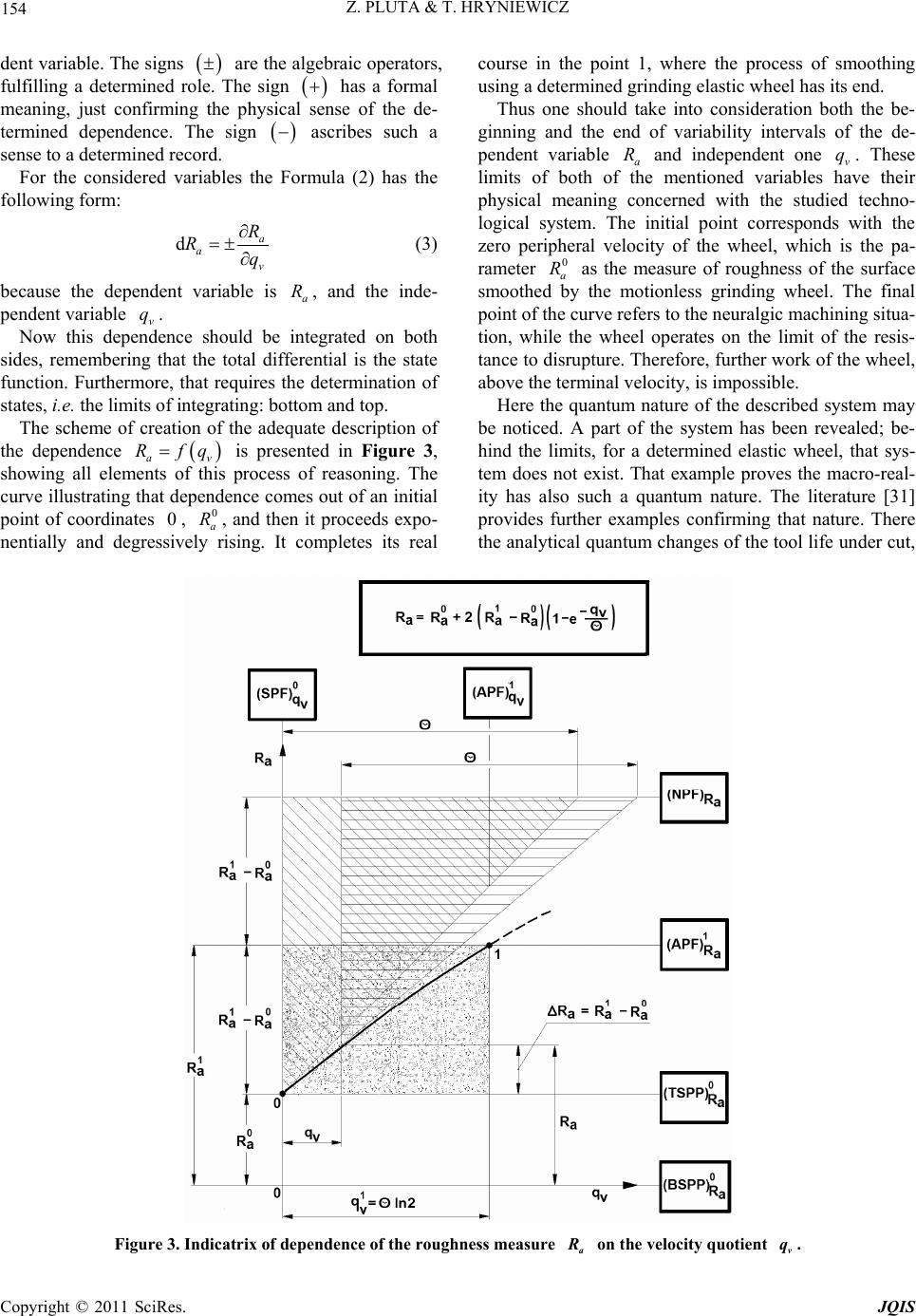

Z. PLUTA & T. HRYNIEWICZ
154
dent variable. The signs are the algebraic operators,
fulfilling a determined role. The sign has a formal
meaning, just confirming the physical sense of the de-
termined dependence. The sign ascribes such a
sense to a determined record.






course in the point 1, where the process of smoothing
using a determined grinding elastic wheel has its end.
Thus one should take into consideration both the be-
ginning and the end of variability intervals of the de-
pendent variable a and independent one v. These
limits of both of the mentioned variables have their
physical meaning concerned with the studied techno-
logical system. The initial point corresponds with the
zero peripheral velocity of the wheel, which is the pa-
rameter as the measure of roughness of the surface
smoothed by the motionless grinding wheel. The final
point of the curve refers to the neuralgic machining situa-
tion, while the wheel operates on the limit of the resis-
tance to disrupture. Therefore, further work of the wheel,
above the terminal velocity, is impossible.
R q
0
a
R
For the considered variables the Formula (2) has the
following form:
da
v
R
q


a
R (3)

because the dependent variable is , and the inde-
pendent variable .
a
R
v
Now this dependence should be integrated on both
sides, remembering that the total differential is the state
function. Furthermore, that requires the determination of
states, i.e. the limits of integrating: bottom and top.
q
Here the quantum nature of the described system may
be noticed. A part of the system has been revealed; be-
hind the limits, for a determined elastic wheel, that sys-
tem does not exist. That example proves the macro-real-
ity has also such a quantum nature. The literature [31]
provides further examples confirming that nature. There
the analytical quantum changes of the tool life under cut,
The scheme of creation of the adequate description of
the dependence av is presented in Figure 3,
showing all elements of this process of reasoning. The
curve illustrating that dependence comes out of an initial
point of coordinates , , and then it proceeds expo-
nentially and degressively rising. It completes its real

q
0
a
R
Rf
0
Figure 3. Indicatrix of dependence of the roughness measure a
R
on the velocity quotient .
v
q

Z. PLUTA & T. HRYNIEWICZ 155
the changes dependent on the main velocity, being the
sta
tool or the workpiece velocities, have been presented.
The mentioned limits, concerning the studied techno-
logical system, are the potential fields. These fields are
situated on two directions; one of them is the direction of
changes of the parameter a
R, whereas the second one is
the direction of changes of the velocity quotient, that is
v
q. On the first direction there are: bottom roughness
ble potential field

0
a
R
BSPF , top roughness stable
potential field

0
a
R
TSPF ness unstable potential , rough
field

1
a
R
APF , an nominal roughness potential d the
field

a
R
NPF . On the second direction there are the
following fields: quotient stable potential field

0
SPF ,
v
q
quotient unstable potential field

1
v
q
A
PF . Bete ween th
fields

0
a
R
BSPF and

0
a
R
TSPF s a potential there i
band.

The fields

0
a
R
TSPF

1
,

a
R
APF, and

0
SPF
v
q
and

1
v
q
A
PF delim, it the interstate space (dotted area)
wheronential and degressively rising changes of e the exp
the parameter a
R take place.
The curve of roughness measure, comprised between
the points 0 - 1, is the envelope of the right-angled trian-
gles, moving with its horizontal leg on the nominal po-
tential field

a
R
NPF ; with the horizontal leg being
invariable and the nominal quotient constant Θ,
and the vertical leg changing respectively, decreasing
with the displacing triangle in the direction of the veloc-
ity quotient. That nominal field is situated symmetrically
against the level of the end of the described system, on
the distance equal the length of the real space-time in the
direction of the surface roughness measure.
Therefore over the real (proper) space there is an im-
pr
equal to
oper space situated, where the curve (dashed line) ap-
proaches towards the asymptote, being the mentioned
potential field. This creation forms an auxiliary design,
required to the description of the real curve, reflecting
the adequate dependence of a R on v q.
Now one may begin to intate thEquation (3), and
in fact
egre
only one of its version, regarding the sign



; it
concerns the analyzed course of the parameter R, that
is the course indeed exponential, but rising degreively,
where the increments of the studied roughness parameter
decrease, respectively. Therefore
a
ss
dd
a
R
Rq


av
v
q  (4)
By integrating the Equation (4), one has to denote the
limits of integrals of the total differentials. That means


110
0
dd
a
av
Rq
q

aaa v
v
aa
RRR q
vq
RR
R
 



 (5)
and further

10 d
2d
a
aa a
v
R
RR Rq

  (6)
or

10
d1d
2
a
v
aa a
Rq
RR R

 (7)
One may notice the partial derivative h
tuted by the quotient of the regular total differentials. It
co
as been substi-
uld be done that way as the regular total differentials
have been distinctly determined by introducing the limits
of their integrals.
Furthermore, by intergrating both sides of the Equa-
tion (7), one obtains the result

10 *
1
ln 2aa a RR RqC

v

 

(8)

that is

**
10
2eeee
vvv
qq
CC
aa a
RR RC
 
q


  (9)
After taking into account that for the magni-
tude
0
v
q
0
a
R

, one obtains


10
2aa CRR (10)
and astituting (10) t fter subo (9), and then, regarding
a
0
aa
RRR



010
21e
v
q
RR RR

 

(11)
aa aa


Now one may determine the second coo
point 1, that is. It is obtained by introducing the pa-
ra
(12)
an
rdinate of the
1
v
q
meter a
R and the mentioned coordinate v q to the
Equation (11).
Thus
1
1 1
ln 2
v
q
d
1
ln 2
v
q
 (13)
Therefore the Equation (11) is
cally for
determined mathemati-
0,
v
q

 , whereas physically for
1
0,
vv
q. Furthermore, however, that equation is not
adjusted to the practical usage because it co
q
ntains a
nominal quotient constant; placed on the nominal field,
being the asymptote, with that improper (mathematic)

Z. PLUTA & T. HRYNIEWICZ
156
he
part of the curve of the parameter a R approaching it. It
should be expressed as a function of its real quotient
constant *
. That dependence may derived by taking
advantage of the scheme (Figure 4).
From t Thales of Milesios theorem the following
proportion results
be

*

10
10
2aa
aa RR
RR

 (14)
so
(15)
and
*
2
*
2

 (16)
and after regarding the dependence (13)
1
*
2ln2
v
q
 (17)
and
(18)
Thus, after substituting (15) to (
1*
2ln2
v
q
11), one obtains

*
010 2
21e
v
q
aa aa
RR RR



  (


19)
And then the equation is adjusted to the
where the adequate characteristics of the studied system
ex
real space,
ist.
Figure 4. Auxiliary scheme to the derivation of dependence
between the nominal and real quotient constant.
Ta d theory, first of all one
hould determine the values of coordinates , with the
*

4. Statistic Elaboration of Results of
Experimental Studies
king advantage of the presente
s* qv
coordinates determining the position of the straight line,
tangent to the searched, adequate course of the parameter
a
R. These coordinates result from the Formula (17), then
1
*v
v
q
q (20)
2ln2
The calculation results of these
indicate that they are lower in values than the experi-
m
where the symbol denotes th
coordinates (Table 2)
ental coordinates.
The values *
v
q should be now elaborated statistically
by approximating them according to the dependence
0*
0 aa v
RRkq (21)
0
k
he in
(m
e initial coefficient of
intensity (rate) of tcrement a
R, that is the surface
roughness measure ean arithmetic profile deviation
from the mean line). That coefficieis with the same the
first derivative of the function

av
Rfq for 0
v
q
nt

,
then
0
0
d
dv
a
vq
R
kq



(22)
For the general written linear dependence of this type
yabx

 (23
oefficients a and b are dete
)
the c
following formulae:
rmined according to the

111
2
2
11
nnn
niiii
iii
nn
ii
ii
xyx y
b
nx x









(24)
Table 2. Results of measurements and calculations of the
magnitude characterizing the studied technological reality.
af, mm/d·str. af, mm/d·str.
0.1 0.2
Ra, µm
qv
Ra, µm
qv *
v
q *
v
q
0.175 105 76 105 76 0.37
0.21 157.5 113 157.113
0. 236.
427.
0.49 5
0.28 210 151 0.53 210 151
245 236.25 170 0.60 25 170
0.35 315 227 0.77 315 227
0.42 420 302 0.98 420 302
0.42 427.5 308 0.91 5 308
0.49 630
0.56 945
453
680
1.19
1.47
630
945
453
680

Z. PLUTA & T. HRYNIEWICZ
157
11i
b

1n 
n
ii
ayx




5)
with the formulae being the result of us
least sum of the deviations squares of
i
n


 (2
ing the rule of the
experimental and
theoretical values, resulting from the position of linear
regression function. That rule is described in detail in the
literature, e.g. [32-35].
The comparison of the magnitudes needed to calculate
the values of the coefficients of the linear regression:
initial roughness parameter a
R and the initial coeffi-
cient of intensity (rate) of the increment of a
R in the
Formula (21) is presented in Table 3.
The coefficient is described by the following formu-
lae:
0




 
**
nnn
vav a
ii
ii
nq RqR

11
1
02
2
**
11
iii
nn
vv
ii
ii
k
nq q






(26)


0*
0
11
1nn
aa
ii
ii
RRkq
n





v
(27)
Thus for mm/d·str. 0.1
f
a

4
02
9 2480
9 1059.3824803.156.55 10
975452
k

 μm (28)

04
13.156.55 1024800.17
9
a
R  μm (29)
Therefore
(30)
By substituting the terminal limit va
0.
4*
0.176.55 10
av
Rq


lue of a
R, that is
56 μm to the Equation (30), one obtains
**
595
v
q . Thus 2595 1190

 , thlts
fromla (15). T) may be now
presented in the quantitative form, by introducing the
values 00.17
a
R μm, 10.56
a
R μm, and 595
at resu
the Formuhe dependence (11


to it. Therefore
1190
0.170.78 1
v
q
a
Re
 
 




(31)
That has been also presented graphically (Figure 5).
That is a quantitative dependence of the roughness mea-
sure a R on the velocity quotient v q for the in-feed
0.1
f
a

mm/d·str.
Furtrmore, for 0.2hef a

mm/d·str.

4
02
9 2555.223118.52k

2480 710
9 9754522480


 μm (32)

04
17.31 18.52 1024800.30
9
a
R  μm (33)
Therefore
(34)
By substituting the terminal limit valu
1.
4*
0.3018.52 10
av
Rq

 
e of a R, that is
47 μm to the Equation (34), one obtains
**
632
v
q . Thus 2 6321264

 , thlts
from
at resu
Table 3. Comparison of magnitudes needed to calculat
the Formula (15). T) may be now
presented in the quantitative form, by introducing the
e the values of coefficients of linear regression.
he dependence (11
af, mm/d·str. af, mm/d·str.

ai
R
0.1 0.2
, µm


*
vi
q

2
*
vi
q



*
va
i
i
qR


ai
R
, µm


*
vi
q

2
*
vi
q



*
va
i
i
qR
i
1 0.175 76 5776 13.30 0.37 76 5776 28.12
2 0.21 113 12769 23.73 0.49 113 12769 55.37
3 0.28 151 22801 42.28 0.53 151 22801 80.03
4 0.245 170 28900 41.65 0.60 170 28900 102.00
5 0.35 227 51529 79.45 0.77 227 51529 174.79
6 0.42 302 91204 126.84 0.98 302 91204 295.96
7 0.42 308 94864 129.36 0.91 308 94864 280.28
8 0.49 453 205209 221.97 1.19 453 205209 539.07
9 0.26 380 462400 380.80 1.47 680 462400 999.60
 3.15 2480 975452 1059.38 7.31 2480 975452 2555.22

Z. PLUTA & T. HRYNIEWICZ
158
a
R
Figure 5. Dependence of roughness measure on the
velocity quotient for the in-feed ·str.
v
q0.1
f
amm/d
values 00.30
a
R μm, 11.47
a
R μm, and 1264


to it. Therefore
1264
0.30 2.34
v
q
a
R 1 e

 



(35)
That has been also presented graphi
That is a quantitative dependence of the
sure
presented material the rules of using of
tic grinding wheels are not the same,
cally (Figure 6).
roughness mea-
a R on the velocity quotient v q for the in-feed
0.2
f
a mm/d·str.
5. Summary
It results from the
the compact elas
congruent to the rules relating to the rational exploitation
of the ceramic wheels. These rules are in fact reversal
and cannot be a criticless copy of the rules of grinding
using the mentioned ceramic wheels. It is important not
to follow the groundless technological imitation, relying
on the equality of the two operations: smoothing/flexible
grinding and a conventional grinding.
Thus, as it has been indicated, to obtain the advanta-
geous finishing results by machining using the elastic
grinding wheel, the possibly least values of the velocity
quotient should be used; contrary to the grinding using a
ceramic wheel where the direction of the value changes
of this parameter should be reversal. That is quite a
valuable observation; knowing that it is not necessary to
a
R
Figure 6. Dependence of roughness measure on the
velocity quotient for the in-feed ·str.
manufacture the elastic wheels of such numerous a d
differentiated sizes of the abrasive grain. The effect
g wheel
v
q0.2
f
amm/d
n
of
the size of this component of the wheel is essential only
in case of grindinusing the ceramics.
It is worthy underlining the presented and completely
solved the quest of elaboration of the experimental mate-
rial, the sets of points of the coordinates being the veloc-
ity quotient and a determined surface roughness measure,
respectively. The introduced quantitative dependences
have a physical meaning which is their essential attri-
bute.
That type of courses, degressively rising, are charac-
teristic for many different systems; they have no analyti-
cal and uniform physical description. The courses do not
possess a separate interval of the physical definition,
turning towards the asymptote, and that is possible only

Z. PLUTA & T. HRYNIEWICZ 159
hus commonly used parabolic regres-
si
may be used with a success to the approxim
of
anical Polishing of Metals,” W
Warszawa, 1968.
amentals of Surface Smoothing Using Elea-
sic Grinding Wheels,” Wydawnictwo Politechniki Kosza-
heel for Polishing and Micro-Chips
cki, Po-
mme of Kronem-R-Flex Abrasives,” Prospectus
Abrasive Materials. Delivery Programme
ed Grinding Fundamental
High Peripheral Velocities
e, and Ero-
Annals of
CIRP, Vol. 23, No. 1, 1974, pp. 103-104.
sive Tools of Porous Elastic Bonds,”
rasive Tools of
on the Surface Quality,” Werkstatt und
ed from Post-Copper Slag,” Werkstatt und
Trennen, Vol.
ternational
in mathematics.
There are some new achievements of the presented
work. Firstly, it is the quantitative approach to the effect
of velocity quotient on the roughness measure of ma-
chined surface. T
Post
on, relying on substitution of the multiple experimental
points has been abandoned. It was discovered that a sig-
nificant decrease of velocity quotient leads to the essen-
tial influencing roughness of the treated material. More-
over, the presented model may have a broader applica-
tion.
It results that the presented here the method of elabo-
ration of sets of experimental points, with the system
indicating their exponential and degreessively rising
course, ation 107, No. 2, 1983, pp. 7-11.
[20] S.-S. Cho, Y.-K. Ryu and S.-Y. Lee, “Curved Surface
Finishing with Flexible Abrasive Tool,” In
experimental material, characterizing also other phe-
nomena or processes.
6. References
[1] M. Rodziewicz, “MechNT,
[2] Z. Pluta, “Fund
lińskiej, Koszalin, 2007.
[3] “‘Soft’ Grinding W
Removal,” Prospectus of SLIP-NAXOS, 2000.
[4] “Elastic Grinding Wheels,” Catalogue of ARTIFEX,
1999.
[5] “Elastic Polishing Wheels,” Prospectus of Grinding
Wheels Manufacture of Grodzisk Mazowie
land, 1998.
[6] “Progra
of KLINGSPOR, 2001.
[7] “Grinding and Polishing,” Catalogue of LUKAS, 2002.
[8] “Systems of ,”
Catalogue of 3M, 1997.
T. Sierżant, E. Weiss and Z.[9] Weiss, “Selected Problem
of High-Speed Grinding,” Biuletyn Techniczny, Vol. 19
s
,
No. 9-10, 1975, pp. 109-114.
[10] F. I. Klocke, “High-Spes and
State of the Art in Europe, Japan and the USA,” Annals of
the CIRP, Vol. 46, No. 2, 1977, pp. 715-724.
[11] “Grinding with Elastic Bond.
Favour Effectiveness of Machining,” Maschinen und Wer-
kzeug, Vol. 100, No. 1-2, 1999, pp. 44-45.
[12] J. Kaczmarek, “Fundamentals of Chip, Abrasiv
sive Treatment,” WNT, Warszawa, 1970.
[13] L. Burnat, “Grinding and Superfinish of Metals,” WNT,
Warszawa, 1962.
[14] M. Kieda, A. Hamada and S. Shiratori, “Polishing of Sili-
con Single Crystals with an Elastic Wheel,”the
[15] Z. Pluta and K. Woźniak, “Some Aspects of Manufacture
and Use of Abra
ępy Technologii Maszyn i Urządzeń, Vol. 7, No. 3,
1983, pp. 39-56.
[16] K. Woźniak, “Manufacture of Elastic Ab
Polyurethane Bonds,” Chemik, Vol. 35, No. 11-12, 1982,
pp. 137- 141.
[17] Z. Pluta, “Effect of Machining Parameters using Elastic
Grinding Wheels
Betrieb, Vol. 7, No. 6, 1988, pp. 487-489.
[18] Z. Pluta and K. Woźniak, “Cutting Ability with Abrasive
Grains Obtain
Betrieb, Vol. 121, No. 10, 1988, pp. 843-847.
[19] W. Kacalak and Z. Pluta, “Grinding and Polishing Using
Elastic Abrasive Wheels,” Schleifen und
Journal of Machine Tools Manufacture, Vol. 42, No. 2,
2002, pp. 229-236. doi:10.1016/S0890-6955(01)00106-7
[21] S. Makuch and W. Kacalak, “The Elastic Properties of
the Flexible Grinding Tools with Polyurethane Bonds,”
Advances in Manufacturing Science and Technology, Vol.
30, No. 1, 2006, pp. 89-99.
[22] Z. Pluta and T. Hryniewicz, “Verification of Forecasts on
Surface Finishing Results of Peripheral Smoothing,” In-
ternational Journal of Advanced Manufacturing Tech-
nology, Vol. 42, No. 5-6, 2009, pp. 515-522.
doi:10.1007/s00170-008-1616-0
[23] Z. Pluta and T. Hryniewicz, “Initial Cutting Conditions
by Abrasive Grain Fixed Flexibly,” International Journal
of Advanced Manufacturing Technology, Vol. 43, No. 5-6,
2009, pp. 440-448. doi:10.1007/s00170-008-1722-z
[24] Z. Pluta, “Butt-Mounted Elastic Wheel,” Utility Pattern
tility
nd Device to Smooth External Ro-
, Vol. 64, No. 3, 1991, pp.
ur Metals,”
the Surface Roughness Smoothed by the
RP No. 55144, 1997.
[25] Z. Pluta, “Mounting to Fix Flat Abrasive Wheels of High
Susceptibility,” Patent RP No. 171852, 1997.
[26] Z. Pluta and A. Markiewicz, “Elastic Wheels,” U
Pattern RP No. 53832, 1996.
[27] Z. Pluta, “The Way a
tary Surface with a Disk-Type Grinding Wheel of High
Susceptibility,” Patent RP No. 168170, 1996.
[28] Z. Pluta, “The Effect of Bond Kind on Some Properties
of Elastic Wheels,” Mechanik
110-116.
[29] K. Woźniak and Z. Pluta, “Use of Elastic Abrasive
Wheels of Post-Copper Slag to Polish Colo
Werkstatt und Betrieb, Vol. 120, No. 1, 1987, pp. 55-58.
[30] Z. Pluta and K. Woźniak, “The Effect of Machining Para-
meters on
Grinding Wheels of Porous Elastic Bonds,” Postępy Tech-
nologii Maszyn i Urządzeń, Vol. 11, No. 1-2, 1987, pp.
45-58.
[31] Z. Pluta and T. Hryniewicz, “Advanced Model of the Tool
Edge Blunting under Machining,” International Journal of
Advanced Manufacturing Technology, Vol. 51, No. 1-4,

Z. PLUTA & T. HRYNIEWICZ
160
2010, pp. 35-43. doi:10.1007/s00170-010-2595-5
[32] K. Mańczak, “Technique of Experiment Planning,” WNT,
Warszawa, 1976.
Introduction to Scientific Studies,” 2nd
“Statistical Adjustment of Data,” Wiley,
ist of More Important Notations
[33] H. Szydłowski, “Theory of Measurements,” PWN, Wars-
zawa, 1978.
[34] E. B. Wilson Jr., “
Edition, PWN, Warszawa, 1968.
[35] W. E. Deming,
New York, 1938.
L*

—real quotient constant

0
BSPF —bottom roughness stable potential field
a
R
f
a—in-feed

a
0
v—velocity in the feed motion
R
TSPF —top roughness stable potential field
p
v—peripheral velocity of the grinding wheel
rowth of
s

1
a
R
APF —roughness unstable potential field
v
k
q—velocity quotient
—initial coefficient of intensity of the g
oughness


a
R
NPF —nominal roughness potential field
0
measure of the surface r

0
v
q
SPF
1
a
R—surface roughness measure (mean arithmetic pro-
file deviation from the mean line)
—quotient stable potential field

v
q
A
PF —quotient unstable potential field
—nominal quotient constant 