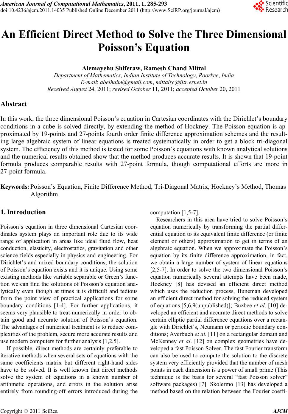
American Journal of Computational Mathematics, 2011, 1, 285-293
doi:10.4236/ajcm.2011.14035 Published Online December 2011 (http://www.SciRP.org/journal/ajcm)
An Efficient Direct Method to Solve the Three Dimensional
Poisson’s Equation
Alemayehu Shiferaw, Ramesh Chand Mittal
Department of Mat hematics, Indian Institute of Technology, Roorkee, India
Received August 24, 2011; revised October 11, 2011; accepted October 20, 2011
Abstract
In this work, the three dimensional Poisson’s equation in Cartesian coordinates with the Dirichlet’s boundary
conditions in a cube is solved directly, by extending the method of Hockney. The Poisson equation is ap-
proximated by 19-points and 27-points fourth order finite difference approximation schemes and the result-
ing large algebraic system of linear equations is treated systematically in order to get a block tri-diagonal
system. The efficiency of this method is tested for some Poisson’s equations with known analytical solutions
and the numerical results obtained show that the method produces accurate results. It is shown that 19-point
formula produces comparable results with 27-point formula, though computational efforts are more in
27-point formula.
Keywords: Poisson’s Equation, Finite Difference Method, Tri-Diagonal Matrix, Hockney’s Method, Thomas
Algorithm
1. Introduction
Poisson’s equation in three dimensional Cartesian coor-
dinates system plays an important role due to its wide
range of application in areas like ideal fluid flow, heat
conduction, elasticity, electrostatics, gravitation and other
science fields especially in physics and engineering. For
Dirichlet’s and mixed boundary conditions, the solution
of Poisson’s equation exists and it is unique. Using some
existing methods like variable separable or Green’s func-
tion we can find the solutions of Poisson’s equation ana-
lytically even though at times it is difficult and tedious
from the point view of practical applications for some
boundary conditions [1-4]. For further applications, it
seems very plausible to treat numerically in order to ob-
tain good and accurate solution of Poisson’s equation.
The advantages of numerical treatment is to reduce com-
plexities of the problem, secure more accurate results and
use modern computers for further analysis [1,2,5].
If possible, direct methods are certainly preferable to
iterative methods when several sets of equations with the
same coefficients matrix but different right-hand sides
have to be solved. It is well known that direct methods
solve the system of equations in a known number of
arithmetic operations, and errors in the solution arise
entirely from rounding-off errors introduced during the
computation [1,5-7].
Researchers in this area have tried to solve Poisson’s
equation numerically by transforming the partial differ-
ential equation to its equivalent finite difference (or finite
element or others) approximation to get in terms of an
algebraic equation. When we approximate the Poisson’s
equation by its finite difference approximation, in fact,
we obtain a large number of system of linear equations
[2,5-7]. In order to solve the two dimensional Poisson’s
equation numerically several attempts have been made,
Hockney [8] has devised an efficient direct method
which uses the reduction process, Buneman developed
an efficient direct method for solving the reduced system
of equations.[5,6,9(unpublished)]; Buzbee et al. [10] de-
veloped an efficient and accurate direct methods to solve
certain elliptic partial difference equations over a rectan-
gle with Dirichlet’s, Neumann or periodic boundary con-
ditions; Averbuch et al. [11] on a rectangular domain and
McKenney et al. [12] on complex geometries have de-
veloped a fast Poisson Solver. The fast Fourier transform
can also be used to compute the solution to the discrete
system very efficiently provided that the number of mesh
points in each dimension is a power of small prime (This
technique is the basis for several “fast Poisson solver”
software packages) [7]. Skolermo [13] has developed a
method based on the relation between the Fourier coeffi-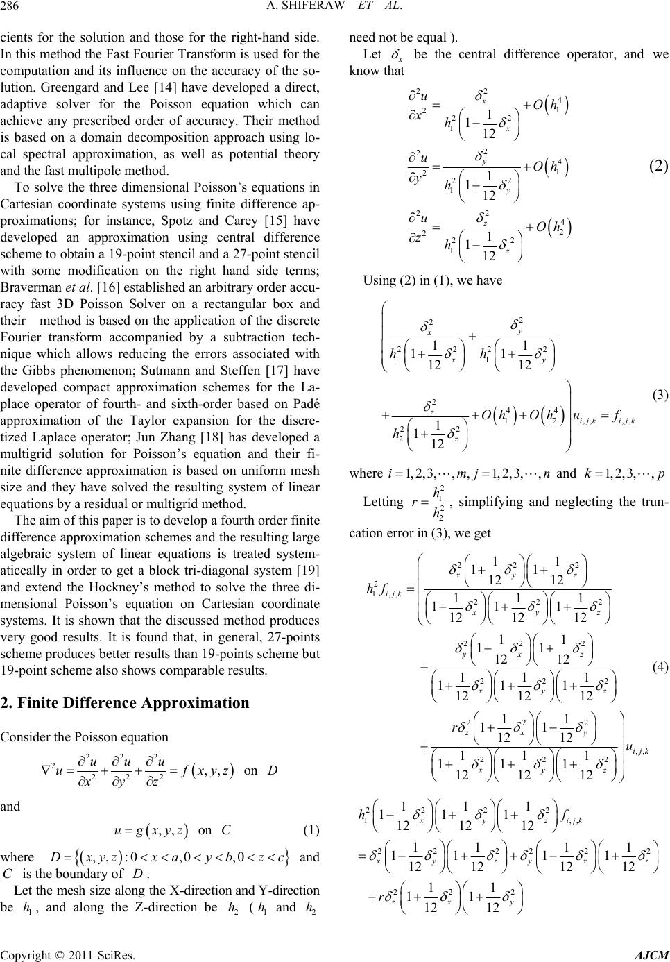

A. SHIFERAW ET AL. 286
cients for the solution and those for the right-hand side.
In this method the Fast Fourier Transform is used for the
computation and its influence on the accuracy of the so-
lution. Greengard and Lee [14] have developed a direct,
adaptive solver for the Poisson equation which can
achieve any prescribed order of accuracy. Their method
is based on a domain decomposition approach using lo-
cal spectral approximation, as well as potential theory
and the fast multipole method.
To solve the three dimensional Poisson’s equations in
Cartesian coordinate systems using finite difference ap-
proximations; for instance, Spotz and Carey [15] have
developed an approximation using central difference
scheme to obtain a 19-point stencil and a 27-point stencil
with some modification on the right hand side terms;
Braverman et al. [16] established an arbitrary order accu-
racy fast 3D Poisson Solver on a rectangular box and
their method is based on the application of the discrete
Fourier transform accompanied by a subtraction tech-
nique which allows reducing the errors associated with
the Gibbs phenomenon; Sutmann and Steffen [17] have
developed compact approximation schemes for the La-
place operator of fourth- and sixth-order based on Padé
approximation of the Taylor expansion for the discre-
tized Laplace operator; Jun Zhang [18] has developed a
multigrid solution for Poisson’s equation and their fi-
nite difference approximation is based on uniform mesh
size and they have solved the resulting system of linear
equations by a residual or multigrid method.
The aim of this paper is to develop a fourth order finite
difference approximation schemes and the resulting large
algebraic system of linear equations is treated system-
aticcally in order to get a block tri-diagonal system [19]
and extend the Hockney’s method to solve the three di-
mensional Poisson’s equation on Cartesian coordinate
systems. It is shown that the discussed method produces
very good results. It is found that, in general, 27-points
scheme produces better results than 19-points scheme but
19-point scheme also shows comparable results.
2. Finite Difference Approximation
Consider the Poisson equation

222
2
222 ,,
uuu
uf
xyz

 
 xyzD


on
and

,,ugxyz on C (1)
where and
is the boundary of .
 
,,:0 ,0 ,0Dxyzxaybzc
D C
Let the mesh size along the X-direction and Y-direction
be , and along the Z-direction be ( and
need not be equal ).
1
h2 h1 h2 h
Let
x

be the central difference operator, and we
know that



2 2
4
1
2
22
1
2
2
4
1
222
1
2 2
4
2
222
1
1
112
1
112
1
112
x
x
y
y
z
z
uOh
xh
uOh
yh
uOh
zh





















(2)
Using (2) in (1), we have
 
2
2
2222
11
2
44
12 ,,,,
22
2
11
11
12 12
1
112
y
x
xy
zijk ijk
z
hh
OhOh uf
h








 







 

 
 

(3)
where 1,2,3, ,,1,2,3, ,imjn


and 1, 2, 3,,kp
Letting
2
1
2
2
h
rh , simplifying and neglecting the trun-
cation error in (3), we get
22 2
2
1,,
222
22 2
222
22 2
11
11
12 12
111
111
12 12 12
11
11
12 12
111
111
12 12 12
11
11
12 12
xy z
ijk
xyz
yx z
xyz
zx y
hf
r
 

 

 






















,,
222
111
111
12 12 12
ijk
xyz
u




 





(4)
22 2 2
1,
22 222
222
111
111
12 12 12
11 11
11 11
12 1212 12
11
11
12 12
xyzijk
xy zyx
zx y
hf
r

,
2
z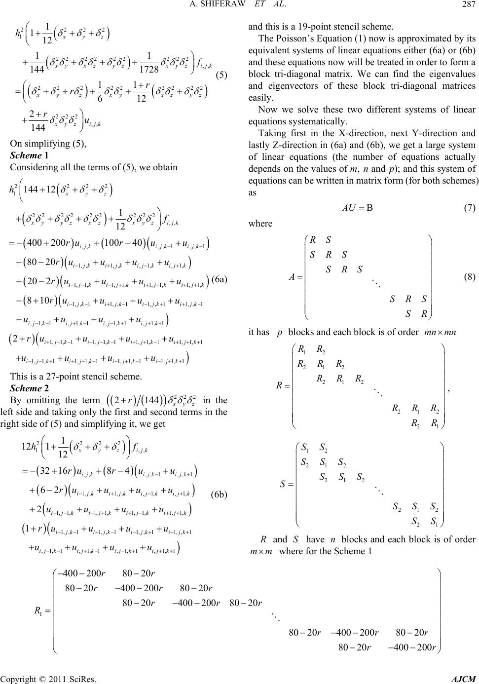








 



 







A. SHIFERAW ET AL. 287


 
2 222
1
22 22 22222
,,
22 2222222
222
,,
1
112
11
144 1728
11
612
2
144
xyz
x
yxzyz xyzijk
xy zxyxzyz
xyz ijk
h
f
r
r
ru

  
 





 









(5)
and this is a 19-point stencil scheme.
The Poisson’s Equation (1) now is approximated by its
equivalent systems of linear equations either (6a) or (6b)
and these equations now will be treated in order to form a
block tri-diagonal matrix. We can find the eigenvalues
and eigenvectors of these block tri-diagonal matrices
easily.
Now we solve these two different systems of linear
equations systematically.
On simplifying (5),
Scheme 1
Considering all the terms of (5), we obtain


 
 

2 222
1
22 22 22222
,,
,,,, 1,, 1
1, ,1, ,,1,,1,
1, 1,1, 1,1, 1,1,
144 12
1
12
400 20010040
8020
202
xyz
xyyzxzxyzijk
ijkijk ijk
ijk ijk ijk ijk
ijkijkijkij
h
f
ruru u
ru uu u
ruuuu

  

 
   




 

 
 
 

 



1,
1, ,11, ,11, ,11, ,1
,1,1,1,1 ,1,1 ,1,1
1, 1, 11, 1, 11, 1, 11, 1, 1
1, 1, 11, 1,11, 1, 1
810
2
k
i jki jki jki jk
ij kijkijkijk
ijk ijk ijk ijk
ijk ijk ijk i
ruuuu
uuuu
ru u uu
uuuu

  
   
  
   
 


  

1, 1, 1jk
(6a)
Taking first in the X-direction, next Y-direction and
lastly Z-direction in (6a) and (6b), we get a large system
of linear equations (the number of equations actually
depends on the values of m, n and p); and this system of
equations can be written in matrix form (for both schemes)
as
AU  (7)
where
RS
SRS
SRS
A
SRS
SR










 (8)
it has blocks and each block is of order
pmn mn

12
212
212
212
21
RR
RRR
RRR
R
RRR
RR










,
This is a 27-point stencil scheme.
Scheme 2
By omitting the term


222
2 144
x
yz
r

  in the
left side and taking only the first and second terms in the
right side of (5) and simplifying it, we get

 
 


2 222
1,,
,,,, 1,, 1
1, ,1, ,,1,,1,
1, 1,1, 1,1, 1,1, 1,
1, ,11, ,11, ,11,
1
121 12
32 1684
62
2
1
xyzijk
ijkijk ijk
ijkijkijkijk
ijkijkijkijk
ijk ijk ijk ij
hf
rur uu
ru u uu
uuuu
ruuuu


 
   
  




  
 
 
 


,1
,1,1 ,1,1 ,1,1 ,1,1
k
ijkijk ijkijk
uuuu

   

(6b)
12
212
212
212
21
SS
SSS
SSS
S
SSS
SS











R
mm
and have n blocks and each block is of order S

where for the Scheme 1
1
400 20080 20
80 20400 20080 20
80 20400 20080 20
80 20400 20080 20
80 20400 200
rr
rrr
rrr
R
rr
rr
 
 
 
 
 
 
 
 
 
 
 
 
 

 

r

A. SHIFERAW ET AL. 288
r
r
2
80 2020 2
2028020 202
2028020202
202 8020202
20 280 20
rr
rrr
rrr
R
rr
rr



 


 



 





1
10040810
8 10100408 10
8 10100408 10
810 10040810
810100 40
rr
rr r
rrr
S
rr r
rr
















2
810 2
28102
28102
28102
2810
rr
rrr
rrr
S
rrr
rr



 


 



 





and for Scheme 2
1
32 1662
623216 62
62321662
6 232166 2
62 3216
rr
rrr
rrr
R
rr
rr
 


 


 



 





2
62 2
262 2
2622
2622
262
r
r
r
R
r
r
















1
841
1841
1841
1841
184
rr
rr r
rr r
S
rr r
rr

















and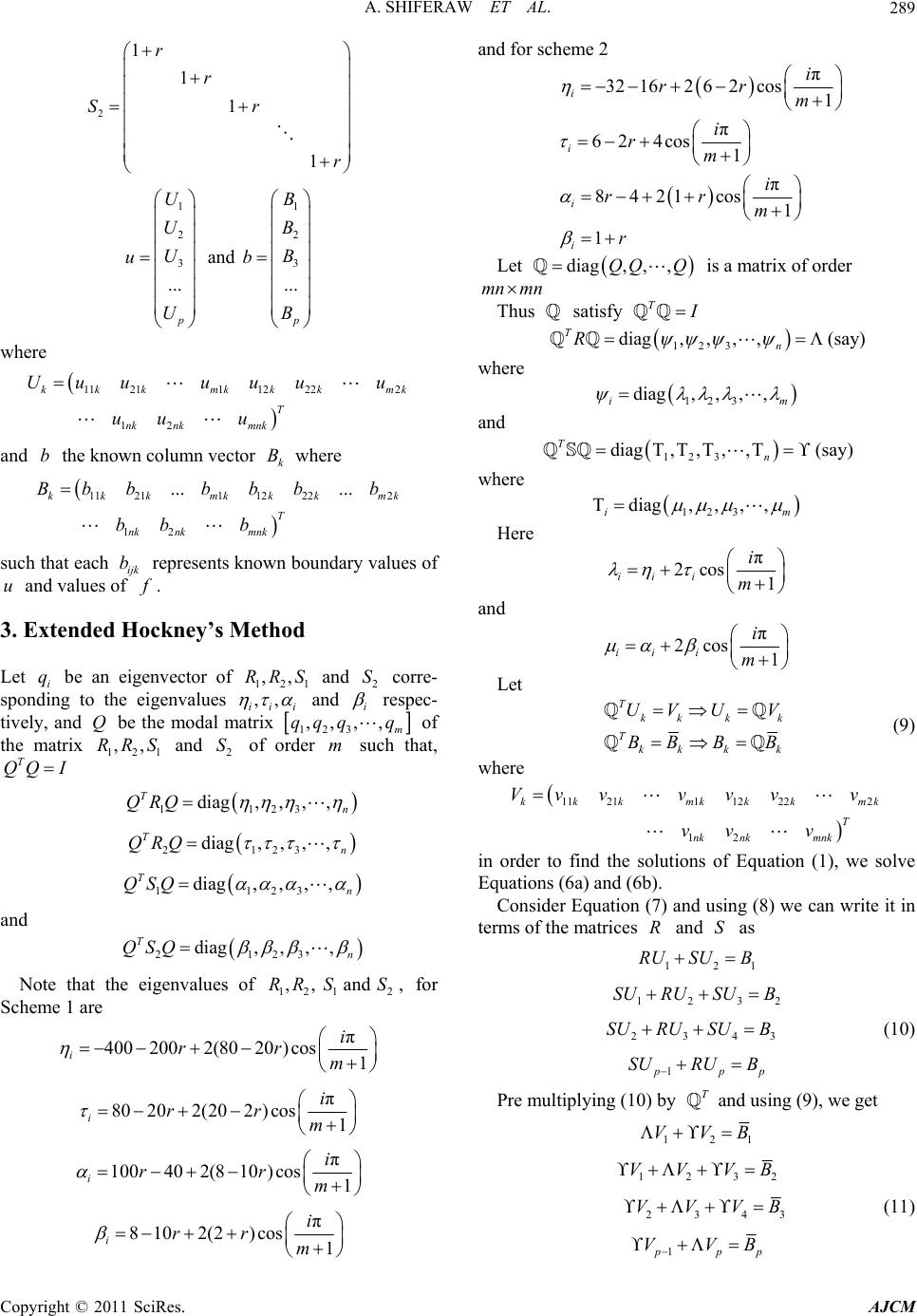

A. SHIFERAW ET AL.289


2
1
1
1
1
r
r
Sr
r













and for scheme 2
1
2
3 and
...
p
U
U
U
u
U








1
2
3
...
p
B
B
B
b
B








where


11211 12222
12
kkkmkkkm
T
nk nkmnk
Uuuu uuu
uu u


k

k
and the known column vector where
bk B


1121112222
12
... ...
kkkmkkkm
T
nk nkmnk
Bbbb bbb
bb b


such that each ijk represents known boundary values of
and values of
b
u
f
.
3. Extended Hockney’s Method
Let i be an eigenvector of and 2 corre-
sponding to the eigenvalues
q121 ,,RRS
,,
ii i
S

 and i

respec-
tively, and be the modal matrix Q


12
,, ,
m
q
m3 of the matrix and of order such that,
,qqq
121
,,RRS2 S
T
QQ I


1123
diag, , ,,
Tn
QRQ

  


2123
diag,, ,,
Tn
QRQ

  


1123
diag,,, ,
Tn
QSQ

  
and


2123
diag,,, ,
Tn
QSQ

 
Note that the eigenvalues of and , for
Scheme 1 are
12 1
,,RR S2 S
π
400 2002(80 20)cos1
ii
rr
m


 


π
80202(202) cos1
ii
rr
m


 


π
100402(810) cos1
ii
rr
m


 


π
810 2(2)cos1
ii
rr
m


  



π
32162 62cos1
ii
rr
m


 


π
62 4cos1
ii
rm 

 



π
8421 cos1
ii
rr
m





1
ir



Let


diag, ,,QQ Q
mn is a matrix order f o mn

Thus  satisfy TI




,,,  
123
diag ,n R 
T

 (say)
where


12 3
diag ,,,,
im

  
and


123
diag,,, ,
Tn

  (say)
where


123
diag,, , ,
im

   
Here
π
2cos 1
ii ii
m
 

 


and
π
2cos 1
ii ii
m
 

 


Let
Tkk k
Tkk k
UV UV
BB BB






k
k
(9)
where


11211 12222
12
kkk mkkkm
T
nk nkmnk
Vvvv vv
vv v


k
v
in order to find the solutions of Equation (1), we solve
Equations (6a) and (6b).
Consider Equation (7) and using (8) we can write in it
terms of the matrices R and S as
121
RU SUB


123
SU RUSBU

2

234
SURU SUB3

 (10)
1
p
pp
SURU B



T
Pre multiplying (10) byand usi ng (9), we get
12
VVB
1

 
1232
VV VB

 
234
VVVB
3

  (11) 
1
p
p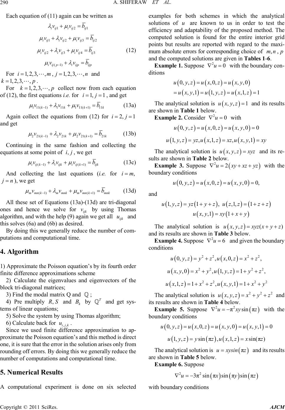p
VV
B

 

A. SHIFERAW ET AL. 290
Each equation of (11) again can be written as
12iij iij ij
vvb  
1
12 32iij iijiijij
vv vb  
23 4iijiijiijij
vvvb   
3
(12)
(1)iij piijpijp
vv 

b
For nan
For collect now from each equation
of s i.e. for , and get
1, 2,3,,im,
2,3,,kp.

1,2, 3,,j d
1,
1,2, 3,,kp
the first equation (12),1, 1ij
1 11(1)1kk
vvvb 

  (13a)
(12) fo
111 11(1)11kk
Again collect the equations fromr 2,1ij


and get
2 21(1)2 212 21(1)21kkkk
Continuing in the same fashion and collecting t
equations
vvvb  
he
at some point of, we get
(13b)
,ij
(1)(1)i ijki ijki ijkijk
And collecting the lasquations (i.e. for ,im
vvvb   
t e
(13c)

jn), we get
(1)(1)mmnkmmnk mmnkmnk
(13a)-(13d) are tri-diag
ce we so
vvv   
All these set of Equations onal
ones and henlve for by using
algorithm, and with the help (9) agwe get a
th
n’s by its fourth order
pproximations scheme
e eigenvalues and eigenvectors of the
algorithm;
for
ce apoxim
irect
on rfrom
ro
es in which the analytical
solutions of are known to us in order to test the
b (13d)
ijk
v
ain
Thomas
ll ijk
u and
is solves (6a) and (6b) as desired.
By doing this we generally reduce the number of com-
putations and computational time.
4. Algorithm
1) Approximate the Poisson equatio
finite difference a
2) Calculate th
block tri-diagonal matrices;
3) Find the modal matrix Q and ;
4) Pre multiply ,RS and k
B by T
 and get sys-
tems of linear equations;
5) Solve the system by using Thomas
6) Calculate back ,,ijk u.
Since we used finite differenpration to ap-
proximate the Poisson equation’s and this method is d
in solution arises only e, it is sure that the erro the
unding off errors. By doing this we generally reduce the
number of computations and computational time.
5. Numerical Results
A computational experiment is done on six selected
examples for both schem
u
efficiency and adaptability of the proposed method. The
computed solution is found for the entire interior grid
points but results are reported with regard to the maxi-
mum absolute errors for corresponding choice of ,mn,p
and the computed solutions are given in Tables 1-6.
Example 1. Suppose 20u

 with the boundary con-
ditions



 
,, 0,,, 0yzuxzuxy

0,u

,,
11,,,1, 1uxyuyzux z


The analytical solution is and its results
are shown in Table 1 below.
Example 2. Consider

,, 1uxyz
20u

 with




,, 0zuxy

0,,, 0,0uyzux






,1, ,1zxy xy1, ,,,,uyzyzuxzux


The analytical solution is and its re-
sults are shown in Table 2
Example 3. Suppose with the
bo

,,uxyzxyz
below.

22uxyxzyz 
undary conditions




0, z
 
,, 00,uxy0, ,,uyzux


and



 

1, ,1,,1,1
,,11
uyz yzyzuzzzz
uxyxyx y


 


The analytical solution is
and its results are shown in Ta
Example 4. Suppose

,, ()uxyzxyzxy z
ble 3 below.
26u

 and given the boundary
conditions


2
0,,, ,,
22 2
, 0

uyzyzxz zux


22 22
,,01,,1,,yxy uyzyz ux


22 2
,1,1,, ,11uxzxz uxyx2 y

 
22
The analytical solution is 2 and
its results are shown in Table 4
Example 5. Suppose z with the
bo

,,uxyz x y
below.
z

22 si πnπuxy
undary conditions




0,,, 0,,, 0uyzuxzuxy
 
, ,10uxy





 
in π,,1, sin(π)zuxzx z 1, ,suyzy
The analytical solution is and its results
are shown in Table 5 belo
Example 6. Suppose

πuxysinz
w.

 
22 sin πsin3πux

πsinzyπ
with boundary conditions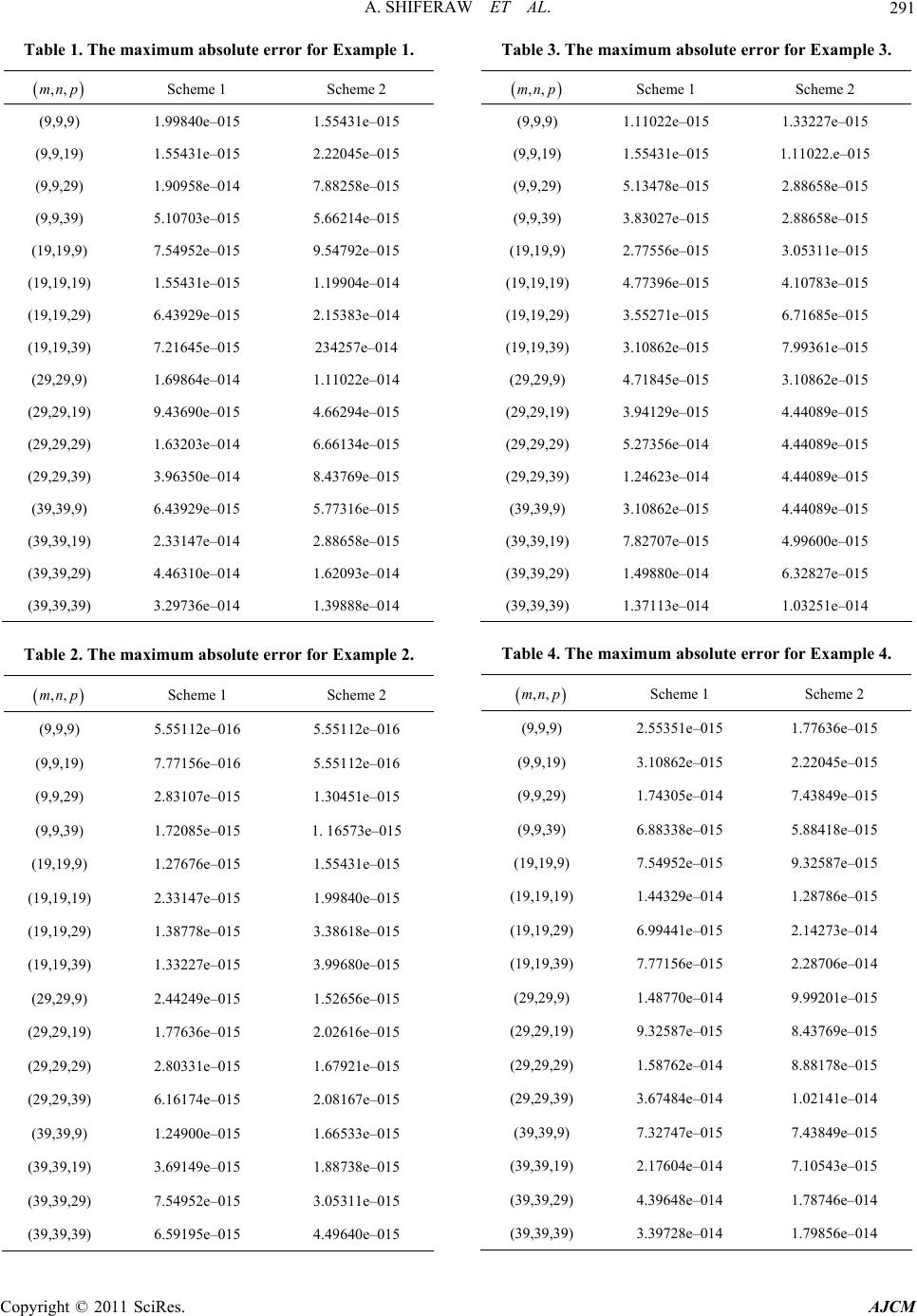

A. SHIFERAW ET AL.291
Table 1. The maximum absolute error for Example 1.
e 1 Scheme 2

,,mnp Schem
(9,9,9) 1.99840e–015 1.55431e–015
(9,9,19)5 2.5
(
1.55431e–0122045e–01
(9,9,29) 1.90958e–014 7.88258e–015
(9,9,39) 5.10703e–015 5.66214e–015
(19,19,9) 7.54952e–015 9.54792e–015
19,19,19) 1.55431e–015 1.19904e–014
(19,19,29) 6.43929e–015 2.15383e–014
(19,19,39) 7.21645e–015 234257e–014
(29,29,9) 1.69864e–014 1.11022e–014
(29,29,19) 9.43690e–015 4.66294e–015
(29,29,29) 1.63203e–014 6.66134e–015
(29,29,39) 3.96350e–014 8.43769e–015
(39,39,9) 6.43929e–015 5.77316e–015
(39,39,19) 2.33147e–014 2.88658e–015
(39,39,29) 4.46310e–014 1.62093e–014
(39,39,39) 3.29736e–014 1.39888e–014
Table 2. The maximum absolute error for Example 2.
Scheme 1 Scheme 2

,,mnp
(9,9,9) 5.55112e–016 5.55112e–016
(9,9,19) 5.
(
7.77156e–01655112e–016
(9,9,29) 2.83107e–015 1.30451e–015
(9,9,39) 1.72085e–015 1. 16573e–015
(19,19,9) 1.27676e–015 1.55431e–015
19,19,19) 2.33147e–015 1.99840e–015
(19,19,29) 1.38778e–015 3.38618e–015
(19,19,39) 1.33227e–015 3.99680e–015
(29,29,9) 2.44249e–015 1.52656e–015
(29,29,19) 1.77636e–015 2.02616e–015
(29,29,29) 2.80331e–015 1.67921e–015
(29,29,39) 6.16174e–015 2.08167e–015
(39,39,9) 1.24900e–015 1.66533e–015
(39,39,19) 3.69149e–015 1.88738e–015
(39,39,29) 7.54952e–015 3.05311e–015
(39,39,39) 6.59195e–015 4.49640e–015
Table 3. The maxrror f. imum absolute eor Example 3


,,mnp Scheme 1 Scheme 2
(9,9,9) 1.11022e–015 1.33227e–015
(9,9,19)5 1.5
(
1.55431e–0111022.e–01
(9,9,29) 5.13478e–015 2.88658e–015
(9,9,39) 3.83027e–015 2.88658e–015
(19,19,9) 2.77556e–015 3.05311e–015
19,19,19) 4.77396e–015 4.10783e–015
(19,19,29) 3.55271e–015 6.71685e–015
(19,19,39) 3.10862e–015 7.99361e–015
(29,29,9) 4.71845e–015 3.10862e–015
(29,29,19) 3.94129e–015 4.44089e–015
(29,29,29) 5.27356e–014 4.44089e–015
(29,29,39) 1.24623e–014 4.44089e–015
(39,39,9) 3.10862e–015 4.44089e–015
(39,39,19) 7.82707e–015 4.99600e–015
(39,39,29) 1.49880e–014 6.32827e–015
(39,39,39) 1.37113e–014 1.03251e–014
e mate error 4. Table 4. Thximum absolu for Example


,,mnp Scheme 1 Scheme 2
(9,9,9) 2.55351e–015 1.77636e–015
(9,9,19) 2.
(
3.10862e–01522045e–015
(9,9,29) 1.74305e–014 7.43849e–015
(9,9,39) 6.88338e–015 5.88418e–015
(19,19,9) 7.54952e–015 9.32587e–015
19,19,19) 1.44329e–014 1.28786e–015
(19,19,29) 6.99441e–015 2.14273e–014
(19,19,39) 7.77156e–015 2.28706e–014
(29,29,9) 1.48770e–014 9.99201e–015
(29,29,19) 9.32587e–015 8.43769e–015
(29,29,29) 1.58762e–014 8.88178e–015
(29,29,39) 3.67484e–014 1.02141e–014
(39,39,9) 7.32747e–015 7.43849e–015
(39,39,19) 2.17604e–014 7.10543e–015
(39,39,29) 4.39648e–014 1.78746e–014
(39,39,39) 3.39728e–014 1.79856e–014

A. SHIFERAW ET AL. 292
Te maxi error f. able 5. Thmum absoluteor Example 5

,,mnp Scheme 1 Scheme 2
(9,9,9) 5.89952e–006 5.90013e–006
(9,9,19) 3.
(
3.67647e–00767666e–007
(9,9,29) 7.25822e–008 7.25853e–008
(9,9,39) 2.29611e–008 2.2962e–008
(19,19,9) 5.92320e–006 5.9233e–006
19,19,19) 3.69122e–007 3.69124e–007
(19,19,29) 7.28734e–008 7.28737e–008
(19,19,39) 2.30532e–008 2.30533e–008
(29,29,9) 5.94508e–006 5.94513e–006
(29,29,19) 3.70486e–007 3.70487e–007
(29,29,29) 7.31427e–008 7.31428e–008
(29,29,39) 2.31384e–008 2.31384e–008
(39,39,9) 5.94513e–006 5.94515e–006
(39,39,19) 3.70489e–007 3.70489e–007
(39,39,29) 7.31432e–008 7.31433e–008
(39,39,39) 2.31386e–008 2.31386e–008
Tabe maximurror fo
Scheme 1 Scheme 2
le 6. Thm absolute er Example 6.

,,mnp
(9,9,9) 4.07466e–005 9.56601e–005
(9,9,19) 3.
(
2.80105e–0059912e–005
(9,9,29) 2.73312e–005 2.79092e–005
(9,9,39) 2.72169e–005 2.35847e–005
(19,19,9) 1.52747e–005 1.01614e–005
19,19,19) 2.53918e–006 5.93387e–006
(19,19,29) 1.85988e–006 3.47172e–006
(19,19,39) 1.74565e–006 2.48652e–006
(29,29,9) 1.3916e–005 3.32432e–006
(29,29,19) 1.18059e–006 1.88497e–006
(29,29,29) 5.01294e–007 1.17049e–006
(29,29,39) 3.87057e–007 7.96897e–007
(39,39,9) 1.36876e–005 7.87013e–006
(39,39,19) 9.52114e–007 6.34406e–007
(39,39,29) 2.72819e–007 5.30167e–007
(39,39,39) 1.58582e–007 3.70168e–007




1,,yzux


, ,0,
,,1
zuz
u xy


 
,1,uxz
 
,, 0xy u
0,uy
0
The analytical solution is




,, sinπxsinπysinπuxyzz

an able 6 above.
This example VI was considered as a test problem in [7]
and [18], and the results show that our meth is more
eme the step
siz
In this work, the three dimensional Poisson’s equation in
systems is approximated by a fourth
order finite difference approximation scheme. Here we
[1] L. Collatz, “The Numerical Treatment of Differential Equa-
r Verlag, Berlin, 1960.
[2] M. K. Jain, “Numerical Solution of Differential Equa-
d its results are shown in T
od
accurate than their methods and in their sch
e is the same for all dimensions but in our case
Z-direction can have a different step length.
6. Conclusions
Cartesian coordinate
used to approximate the Poisson’s equation by a 27-
points scheme and a 19-points scheme, and in doing this
by the very nature of finite difference method for elliptic
partial differential equations, it resulted in transforming
the Poisson’s equation (1) in to a large number of alge-
braic systems of linear Equations (6a) or (6b) which
forms a block tri-diagonal matrix in both schemes. These
block tri-diagonal matrices are quite comfortable to find
the eigenvalues and eigenvectors in order to extend
Hockney’s method to three dimensions, and we have suc-
cessfully reduced matrix A to a tri-diagonal one and by
the help of Thomas Algorithm we solved the Poisson’s
equation. The main advantage of this method is that we
have used a direct method to solve the Poisson’s equa-
tion for which the error in the solution arises only from
rounding off errors; because it’s a direct method the so-
lution of (1) is sure to converge as we are always solving
(1) by transforming it in to a diagonally dominant tri-
diagonal system of linear equations; and it reduces the
number of computations and computational time. It is
found that this method produces very good results for
fourth order approximations and tested on six examples.
Actually it is shown that the discussed method, in gen-
eral, for 27-points scheme produces better results than
19-points scheme but 19-point scheme has also shown
comparable results.
Therefore, this method is suitable to find the solution
of any three dimensional Poisson’s equation in Cartesian
coordinates system.
7. References
tions,” Springe

A. SHIFERAW ET AL. 293
Partial Differential
ew York, 1985.
duction to Numerical Ana-
Equa-
0.321259
tions,” New Age International Ltd., New Delhi, 1984.
[3] R. Haberman, “Elementary Applied
Equations with Fourier Series and Boundary Value Prob-
lems,” Prentice-Hall Inc., Saddle River, 1987.
[4] T. Myint-U and L. Debnath, “Linear Partial Differential
Equations for Scientists and Engineers,” Birkhauser, Bos-
ton, 2007
[5] G. D. Smith, “Numerical Solutions of Partial Differential
Equations: Finite Difference Methods,” Oxford Univer-
sity Press, N
[6] G. H. Golub and C. F. van Loan, “Matrix Computations,”
Johns Hopkins University Press, Baltimore, 1989.
[7] J. Stoer and R. Bulirsch, “Intro
lysis,” Springer-Verlag, New York, 2002.
[8] R. W. Hockney, “A Fast Direct Solution of Poisson
tion Using Fourier Analysis,” Journal of ACM, Vol. 12,
No. 1, 1965, pp. 95-113. doi:10.1145/32125
[9] W. W. Lin, “Lecture Notes of Matrix Computations,” Na-
tional Tsing Hua University, Hsinchu, 2008.
[10] B. L. Buzbee, G. H. Golub and C. W. Nielson, “On Di-
rect Methods for Solving Poisson’s Equations,” SIAM
Journal on Numerical Analysis, Vol. 7, No. 4, 1970, pp.
627-656. doi:10.1137/0707049
[11] A. Averbuch, M. Israeli and L. Vozovoi, “A Fast Pois-
son’s Solver of Arbitrary Order Accuracy in Rectangular
regions,” SIAM Journal on Scientific Computing, Vol. 19,
No. 3, 1998, pp. 933-952.
doi:10.1137/S1064827595288589
[12] A. McKenney, L. Greengard and A. Mayo, “A Fast Pois-
son Solver for Complex Geometries,” Journal of Compu-
tation Physics, Vol. 118, No. 2, 1996, pp. 348-355.
doi:10.1006/jcph.1995.1104
[13] G. Skolermo, “A Fourier Method for Numerical Solution
Direct Adaptive Poisson
of Poisson’s Equation,” Mathe matics of Computation, Vol.
29, No. 131, 1975, pp. 697-711.
[14] L. Greengard and J. Y. Lee, “A
Solver of Arbitrary Order Accuracy,” Journal of Compu-
tation Physics, Vol. 125, No. 2, 1996, pp. 415-424.
doi:10.1006/jcph.1996.0103
[15] W. F. Spotz and G. F. Carey, “A High-Order Compact
-2426(199603)12:2<235::AID-N
Formulation for the 3D Poisson Equation,” Numerical
Methods for Partial Differential Equations, Vol. 12, No.
2, 1996, pp. 235-243.
doi:10.1002/(SICI)1098
UM6>3.0.CO;2-R
[16] E. Braverman, M. Israeli, A. Averbuch and L. Vozovoi,
“A Fast 3D Poisson Solver of Arbitrary Order Accuracy,”
Journal of Computation Physics, Vol. 144, No. 1, 1998,
pp. 109-136. doi:10.1006/jcph.1998.6001
[17] G. Sutmann and B. Steffen, “High Order Compact Solvers
for the Three-Dimensional Poisson Equation,” Journal of
Computation and Applied Mathematics, Vol. 187, No. 2,
2006, pp. 142-170. doi:10.1016/j.cam.2005.03.041
[18] J. Zhang, “Fast and High Accuracy Multigrid Solution of
the Three Dimensional Poisson Equation,” Journal of
Computation Physics, Vol. 143, No. 2, 1998, pp. 449-
461. doi:10.1006/jcph.1998.5982
[19] M. A. Malcolm and J. Palmer, “A Fast Method for Solv-
ing a Class of Tri-Diagonal Linear Systems,” Communi-
cations of the ACM, Vol. 17, No. 1, 1974, pp. 14-17.
doi:10.1145/360767.360777