American Journal of Computational Mathematics, 2011, 1, 256-263
doi:10.4236/ajcm.2011.14031 Published Online December 2011 (http://www.SciRP.org/journal/ajcm)
Context-Dependent Data Envelopment Analysis with
Interval Data
Mohammad Izadikhah
Department of Mat hematics, Islamic Azad University, Arak, Iran
Received August 11, 2011; revised Septembe r 20, 2011; accept ed September 28, 2011
Abstract
Data envelopment analysis (DEA) is a non-parametric method for evaluating the relative efficiency of deci-
sion making units (DMUs) on the basis of multiple inputs and outputs. The context-dependent DEA is intro-
duced to measure the relative attractiveness of a particular DMU when compared to others. In real-world
situation, because of incomplete or non-obtainable information, the data (Input and Output) are often not so
deterministic, therefore they usually are imprecise data such as interval data, hence the DEA models be-
comes a nonlinear programming problem and is called imprecise DEA (IDEA). In this paper the con-
text-dependent DEA models for DMUs with interval data is extended. First, we consider each DMU (which
has interval data) as two DMUs (which have exact data) and then, by solving some DEA models, we can find
intervals for attractiveness degree of those DMUs. Finally, some numerical experiment is used to illustrate
the proposed approach at the end of paper.
Keywords: DEA, Context-Dependent, Interval Data, Interval Attractiveness, Interval Progress
1. Introduction
Data envelopment analysis (DEA), developed by Char-
nes et al. [1], usually evaluates decision making units
(DMUs) from the angle of the best possible relative effi-
ciency. If a DMU is evaluated to have the best possible
relative efficiency of unity, then it is said to be DEA ef-
ficient; otherwise it is said to be DEA inefficient. Per-
formance of inefficient DMUs depends on the efficient
DMUs, that is, the inefficiency sco res change only if the
efficiency frontier is altered.
Although the performance of efficient DMUs is not
influenced by the presence of inefficient DMUs, it is
often influenced by the context. The context-dependent
DEA [2-4] is introduced to measure the relative attrac-
tiveness of a particular DMU when compared to others.
We know that the DMUs in the reference set can be used
as benchmark targets for inefficient DMUs. The con-
text-dependent DEA provides several benchmark targets
by setting evaluation context [3]. The context-dependent
DEA is introduced to measure the relative attractiveness
of a particular DMU when compared to others. Relative
attractiveness depends on the evaluation context con-
structed from alternative DMUs. The original DEA
method evaluates each DMU against a set of efficient
DMUs and cannot identify which efficient DMU is a
better option with respect to the inefficient DMU. This is
because all efficient DMUs have an efficiency score of
one. The standard DEA models assume that all data are
known exactly without any variation. However, this as-
sumption may not be true. In the real world, some out-
puts and inputs may be only known as in forms of inter-
val data, ordinal data and ratio interval data. If we incor-
porate such imprecise data information in to the standard
linear CCR model, the resulting DEA model is a nonlin-
ear and non-convex program, and is called imprecise
DEA (IDEA), (Cooper et al. [5] and Kim et al. [6]). Th e
approach in IDEA is to transform the non-linear and
non-convex model to a linear programming equivalent,
by imposing scale transformation on the data variable
alterations (products of variables are replaced by new
variables). Prior to IDEA, pertinent work was that of
Cook et al. [7,8], which, is confined only to mixture of
exact and ordinal data. They started by dealing with only
one ordinal input [8] and then extended their model [7]
to handle multiple cardinal and ordinal criteria. The basic
idea in these models is to assign new auxiliary variables,
one for every combination of ordinal variables and dis-
tinct ranks of it. The value for such an auxiliary variable
corresponding to DMU
j
and a rank position is 1, if

M. IZADIKHAH257
DMU
j
is rated in the k-th place of ordinal variable and
0 otherwise. Extensions of these basic ideas are reported
in [9,10]. Recently, Despotits and Smirlis [11] calculated
upper and lower bounds for the efficiency scores of the
DMUs with imprecise data. They developed an alterna-
tion approach for dealing with imprecise data. They
transformed the non-linear DEA model to a linear pro-
gramming equivalent by using a straightforward formu-
lation, completely different than that in IDEA. Contrarily
to IDEA their transformation on the variables are made
on the basis of the original data set, without applying any
scale transformations on data. Also, in Jahanshahloo et al.
[12,13] the radius of stability for the DMUs with interval
data is calculated. In this paper we concentrate on the
context-dependent DEA with interval data. For this rea-
son we consider each DMU
j
, with interval data, as two
DMUs that have exact data. Then by a procedure similar
to that one in [3], the evaluation contexts are obtained by
partitioning these DMUs into several levels of efficient
frontier. Then by introducing some models based upon
these efficient frontiers we can measure the relative at-
tractiveness and progress of these DMUs and also we can
determine the interval attractiveness and interval pro-
gress for each original DMU with interval data. Further
by combination of these measures we can also character-
ize the performance of DMUs.
The rest of the paper is organized as follows: next sec-
tion introduces the basic definitions of interval data and
notations of the original context-dependent DEA. In Sec-
tion 3, interval context-dependent DEA is presented. In
Section 4 we illustrate our proposed DEA method with
two numerical examples and some discussion. Finally,
some conclusions are pointed out in the end of this paper.
2. Preliminaries
Now suppose we have DMUs which utilize in-
puts n

m

,1,,
ij
x
imto produce
s
outputs
rj

,1,,,

1,,

y
rs
1
jn

,,
. Also, assume that input
and output levels of each DMU are not known exactly.
We define
j
jmj
X
xx and

1,,
j
jsj
Yy y,
.
1, ,jn
2.1. Interval Data
Let input and output values of any DMU be located in a
certain interval, where
L
ij
x
and U
ij
x
are the lower and
upper bounds of the i-th input of the DMU
j
, respecti-
vely, and
L
rj
y, are the lower and upper bounds of
the r-th output of the
U
rj
yDMU
j
, respectively, that is to say,
L
U
ijij ij
x
xx and
L
U
ry j rj
yy
rj . Such data are called
interval data, because they are located in intervals. Note
that always
L
U
ij ij
x
x and
L
U
rj
y
rj
y. If
L
U
ijij
x
x, then
the i-th input of the DMU
j
has a definite value.
Interval problems are those whose parameter values
are located in intervals, their exact values being unable to
be identified.
Therefore we consider problems with data such as
,
LU
ijij ij
x
xx




 and rj rj
,
LU
y
rj
yy




, where lower and
upper bounds are known exactly, positive and finite.
2.2. Context-Dependent Data Envelopment
Analysis with Exact Data
The original context-dependent DEA model is developed
by using the following radial efficiency measure. Let 1
I
be the set of all DMUs, and k
I
and interactively
defined as
k
E
1kkk
I
IE


, where consists of all the
radially efficient DMUs by following linear program-
ming:
k
E




*
0
0
..
oo
jj
jj o
k
kk
stX X
Yk
jFE





()
()
max
0,
k
k
jFI
jFI
j






Y
(1)
where


k
jFI means DMU k
j
I

E
. When k = 1,
model (1) becomes the original output oriented CCR
model and define the first-level efficient frontier.
When k = 2, model (1) gives the second-level efficient
frontier after the exclusion of the first-level efficient
DMUs. And so on. In this manner we identify several
levels of efficient frontiers. We call the k-th level
efficient frontier.
1
E
k
Assume that, , 0. We can
calculate relative attractiveness measures for
with respect to k-th level efficient frontier. Based upon
the evaluation context , relative attractiveness meas-
ure of o can obtained by the following con-
text-dependent DEA:
0
k
k
E
DMUoE
k
E
0
1, ,kn
DMUo
DMU 




0
0
()
()
ax
0,
kk
kk
oo
E
E


0
*0
0
0
m 1,...,-
..
jj
jF
jj o
jF
kk
j
H
kH
X 



kkL
st X
YHkY
jFE 



k






 (2)
Then




**
o
1
o
A
kHk
DMUo
0, ,k

k
is called the (output oriented)
attractiveness of from a specific level .
k
E
Model (2) is same as [3] with slightly change. In
model (2) we set 0
L

 in order to consider-
ing as evaluation context for .
0
k
E0 DMU k
oE
Note: In this paper, only, attractiveness measure is
used. By the same mann er one can use progress m easure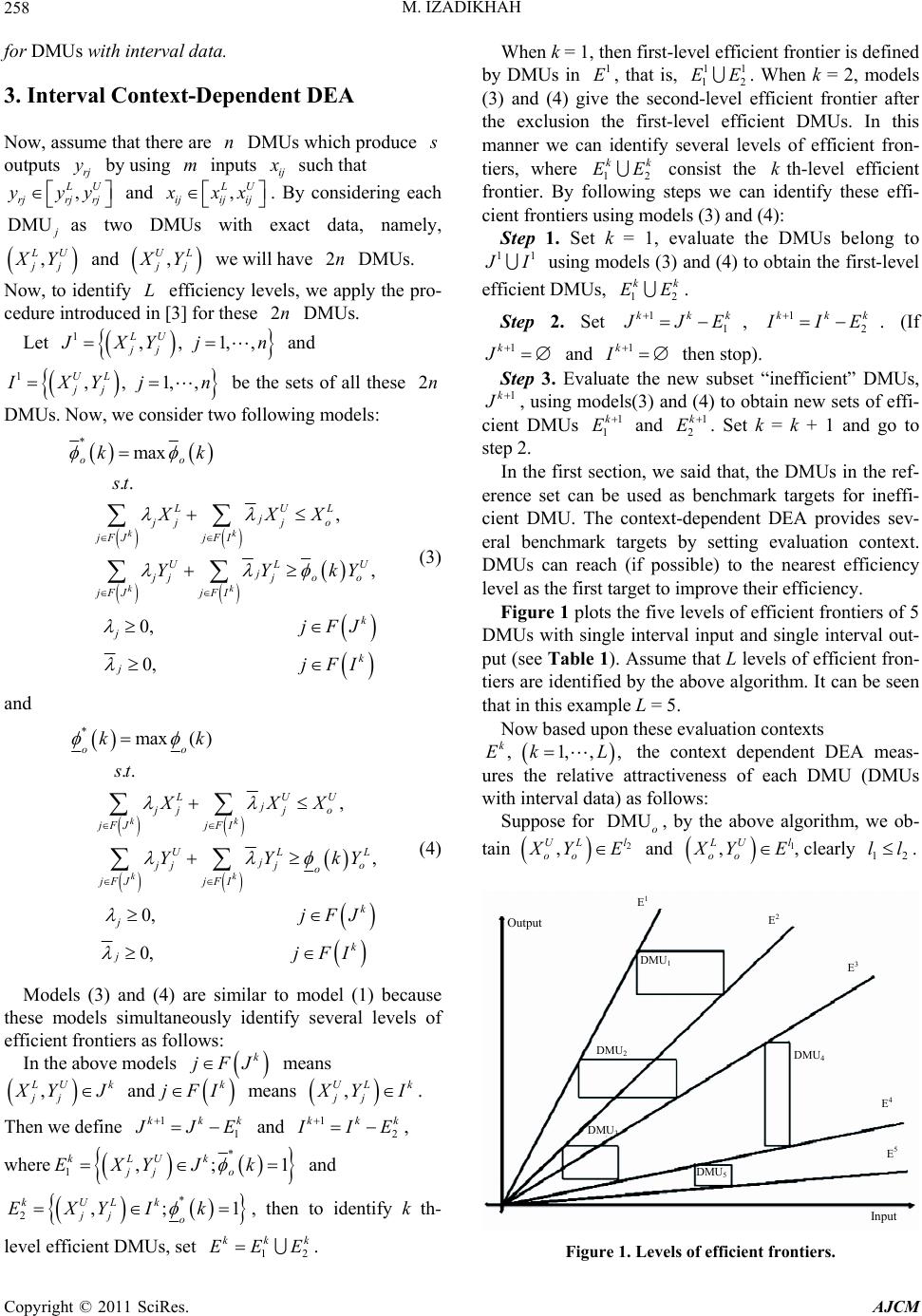

M. IZADIKHAH 258
for DMUs with interval data.
3. Interval Context-Dependent DEA
Now, assume that there are DMUs which produce n
s
outputs by using inputs
rj
ymij
x
such that
,U
rjrj rj
yyy
L


and ,
LU
ijij ij
x
xx


. By considering each
DMU
j
as two DMUs with exact data, namely,

U
,
L
jj
X
Y and

,
UL
j
j
X
Y we will have DMUs. 2n
Now, to identify efficiency levels, we apply the pro-
cedure introduced in [3] for these DMUs.
L2n
Let
 
1,, 1,, LU
jj
J
XY jn
 
,, 1,,
UL
jj
and

1
I
XY jn be the sets of all these
DMUs. Now, we consider two following models:
2n
 
 
 


*max
..
,
,
0,
0,
kk
kk
oo
LUL
j
jjj o
jFJjFI
UL
jo
jjj o
jFJjFI
k
j
j
kk
st
XXX
YYk
jFJ















k jFI
U
Y

(3)
and

 
 


*max()
..
,
,
0,
0,
kk
kk
oo
LUU
j
jjj o
jFJjFI
UL
jL
j
jj
o
jFJjFI
k
j
j
kk
st
XXX
YYk
jFJ















k jFI
o
Y
(4)
Models (3) and (4) are similar to model (1) because
these models simultaneously identify several levels of
efficient frontiers as follows:
In the above models


k
jFJ means

,
L
U
jj k
X
YJ and means

k
jFI

,
UL k
jj
X
YI

.
Then we define 11
kkk
J
JE
 and 12 kkk
I
IE
,
where



*
1,;
kLUk
o jj
EXYJk   1
and



*
2,;
kULk
jj o
EXYIk  

1
k
1
k
1
, then to identify k th-
level efficient DMUs, set .
12
kk
EEE
When k = 1, then first-level efficient frontier is defined
by DMUs in , that is, 2 . When k = 2, models
(3) and (4) give the second-level efficient frontier after
the exclusion the first-level efficient DMUs. In this
manner we can identify several levels of efficient fron-
tiers, where 12 consist the th-level efficient
frontier. By following steps we can identify these effi-
cient frontiers using models (3) and (4):
1
E
E
1
1
EE
k
Ek
Step 1. Set k = 1, evaluate the DMUs belong to
1
J
I using models (3) and (4) to obtain the first-level
efficient DMUs, .
12
kk
EE
Step 2. Set 11
kkk
J
JE
 , 12 kkk
I
IE
 . (If
1k
J

 and 1k I

 then stop).
Step 3. Evaluate the new subset “inefficient” DMUs,
1k
J

, using models(3) and (4) to obtain new sets of effi-
cient DMUs 1
1
k
E

and . Set k = k + 1 and go to
step 2.
1
2
k
E
In the first section, we said that, the DMUs in the ref-
erence set can be used as benchmark targets for ineffi-
cient DMU. The context-dependent DEA provides sev-
eral benchmark targets by setting evaluation context.
DMUs can reach (if possible) to the nearest efficiency
level as the first target to improve their efficiency.
Figure 1 plots the five levels of efficient frontiers of 5
DMUs with single interval input and single interval out-
put (see Table 1). Assume th at L levels of efficient fron-
tiers are identified by the above algorithm. It can be seen
that in this example L = 5.
Now based upon these evaluation contexts


, 1,,,
k
Ek L the context dependent DEA meas-
ures the relative attractiveness of each DMU (DMUs
with interval data) as follows:
Suppose for , by the above algorithm, we ob-
DMUo
tain


2
,
UL
oo l
X
YE and


1
,l
LU
oo
X
YE, clearly 12 ll

.
Output
DMU2
DMU1
DMU3
DMU5
DMU4
E4
E5
E3
E2
E1
Input
Figure 1. Levels of efficient frontiers.

M. IZADIKHAH259
Table 1. Data of numerical example.
DMUj Inputs
L
j
x
U
j
x
Outputs
L
j
y U
j
y
1 3.5 6 6 7
2 2.1 5 3 4.2
3 1.5 3 0.6 1.5
4 7.5 8 1.6 4.5
5 5 6 0.5 1
Now, we introduce two following context dependent
DEA models to obtain the relative attractiveness meas-
ure.
 




22
12
22
12
2
*
2
1
max, 0,,
..
,
,
0,
0,
kl kl
kl kl
oo
LUL
j
jjj o
jFEjFE
UL
o j
jjj o
jFEjFE
kl
j
j
HkHkk Ll
st
XXX
YYH
jFE


















2
2
kl jFE


U
kY
(5)
and
 




22
12
22
12
2
*2
1
max,0,,
..
,
,
0,
0,
kl kl
kl kl
oo
LUU
j
jjj o
jFEjFE
UL
jo
jjj o
jFEjFE
kl
j
j
HkHkk Ll
st
XXX
YYH
jFE


















2
2
kl jFE


L
kY
(6)
Clearly,

*1
o
Hk and


*1
o
Hk for
2
0,, kLl , and also,
 
*
1
o* o
H
kH k and
 
**
1
oo
H
kH k.
Theorem 1. For we have DMUo
 
**,
oo
H
kHk
2
Proof. First assume that
0, ,.kLl


*
*
,,
o
Hk *

 be optimal
solution for model (5). Thus we have




22
12
klkl
ULUL
oo j
j
jjoo
jFEjFE
YYHkYHkY 




therefore


*
*
,, o Hk *

 is a feasible solution for
model (6). Since model (6) is maximization and has an
optimal value as

*
o
H
k, then
 
**
oo
H
kHk.
Corollary 1. If


DMU ,
X
Y has exact data, where
L
U
oo
X
XX and
L
U
o
YYY
o
, then we must have
  
**
*2
,,0,, oo
H
kHkHkk L

l





, where

*
H
k
is the relative attractiveness measure for DMU .
Assume that has interval data, that is,
DMUo
U
o
,
L
oo
XXX




 and ,
LU
ooo
YYY




. By Corollary 1,
  
**
*2
,,0,,
oo.
H
kHkHkk Ll






Definition 1. If we call k-degree attractiveness of
(which is lie on the specific level DMUo
ll
22
1
EEE2
2
l
) by


*
o
A
k, then we h ave
  
***
11
,
o
oo
Ak Hk
H
k









. That is, attractiveness score
of with respect to efficiency level is DMUok E


*
o
A
k.
Definition 2. We define
 
**
11
,
oo
Hk
H
k




as k-de-
gree attractiveness of . DMUo
Since th e parameter v alues are located in intervals and
their exact values being unable to be identified, hence
value of


*
o
A
k is unknown. Also, one can rank the
DMUs in each level based upon their attractiveness
scores.
4. Application
In order to illustrate the use of the methodology for de-
termining the interval attractiveness developed here, first,
in example 1 we use the data in Table 1 and in example
2 we use an empirical data.
4.1. Example 1: Personal Selection Data
Assume that, we have 5 DMUs in one input and one
output and these data are interval as shown in Table 1.
By considering each DMU
j
as two DMUs with exact
data, namely,


U
jj
,
L
X
Y and

,
UL

j
j
X
Y we will have
10 DMUs. Now, to identify the efficient levels of these
DMUs, we apply models (3) and (4).
Results are shown below:







111 22
,,,
LU LU
EXYXY







21133
,,,
UL LU
EXYXY







322 44
,,,
UL LU
EXYXY




 


433 44 55
,, ,,,
UL ULLU
EXYXYXY





555
,
UL
EXY

M. IZADIKHAH 260
We see that for these DMUs, 5 efficient levels are
identified, i.e., = 5. By models (5) and (6), interval
attractiveness of each DMU can be calculated. In Table 2
interval attractiveness of each original DMUs (which
have interval data) are shown in column 4. For example,
in Table 2, first-degree interval attractiveness of
with respect to efficiency level is [1.67, 3.33].
L
1
DMU
3
E
That is, if we choose exact value for input and output
of and then calculate the attractiveness degree
of 1 with respect to efficiency level , namely
, we must have .
1
DMU
DMU
(3)
3
E
*
1
A*
1
1.67(3)3.33A
Discussion
In the above mentioned example, suppose that, we fix the
data of these DMUs in their intervals, in th e other words,
assume that we have 5 DMUs, namely,

DMU,, 1,,5, jj
jXY j which have exact data
such that ,
LU
j
j
j
XXX

 , ,
LU
jjj YYY



. These data
are as Table 3.
We will show that, the attractiveness score of these
DMUs lies in the interval attractiveness presented in Ta-
Table 2. Interval attractiveness.
DMUj k-degree Efficiency Levels k-degree inte rval
attractiveness
1 Zero-degree 2
E [1,2]
First-degree 3
E [1.67,3.33]
Second-degree 4
E [5,10]
Third-degree 5
E [12,24]
2 Zero-degree 3
E [1,3.33]
First-degree 4
E [3,10]
Second-degree 5
E [7.2,24]
3 Zero-degree 4
E [1,5]
First-degree 5 E [2.4,12]
4 Zero-degree 4
E [1,3]
First-degree 5
E [2.4,7.2]
5 Zero-degree 5
E [1,2.4]
Table 3. DMUs with exact data.
DMUj Input Output
1 5 6
2 3 4
3 2 1
4 7.5 4.5
5 6 0.5
ble 2. Hence, we employ models (3) and (4) for these
DMUs. Let k E be the th-level of efficient frontier.
See Figure 2 and compare
kk
E and .
k
E
We define


k
SE as follows:


 
11
,,,0,,
k
nn k
jjjj jjj
jj
SE
x
yxX yYXYE 









For example, Figure 3 illustrates region of


k
SE .
It can be seen that,












54
54 3
321
21
SE SESESESE
SESE SE SESE


Assume that, we want to calculate the attractiveness
degree of 1 DMU with respect to efficiency level 4 E,
that is, we want to calculate . Since

*
14A2
1
DMU E
and




4
34
SE SESE, hence the attractiveness
Output
Input
DMU
1
DMU
2
DMU
3
DMU
5
DMU
4
E
1
E
3
E
4
E
5
5
3
2
1
4
1
E
2
E
E
2
3
E
5
E
Figure 2. Levels of efficient froutiers for DMUs with exact
data and interval data.
Output
Input
3
E


3
SE
Figure 3. Region of

3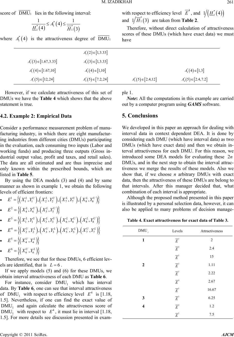
S
E.

M. IZADIKHAH 261
with respect to efficiency level 4 E, and


*
1
14H score of 1 DMU lies in the following interval:
and

*
1
13H are taken from Table 2.
  
*
1
**
11
11
4
43
A
HH
 Therefore, without direct calculation of attractiveness
scores of these DMUs (which have exact data) we must
have
where is the attractiveness degree of

*
14A1
DMU



*
221,3.33A
 

*
13 1.67,3.33A



*
231,3.33A
 

*
141.67,10A



*
241,10A




*
441,3A
 

*
1512,24A



*
257.2,24A




*
352.4,12A
 

*
452.4,7.2A
However, if we calculate attractiveness of this set of
DMUs we have the Table 4 which shows that the above
statement is true.
4.2. Example 2: Empirical Data
Consider a performance measurement problem of manu-
facturing industry, in which there are eight manufactur-
ing industries from different cities (DMUs) participating
in the evalua tion, each consuming two inputs ( Labor and
working funds) and producing three outputs (Gross in-
dustrial output value, profit and taxes, and retail sales).
The data are all estimated and are thus imprecise and
only known within the prescribed bounds, which are
listed in Table 5.
By using the DEA models (3) and (4) and by same
manner as shown in example 1, we obtain the following
levels of efficient frontiers:



  
11122 77 88
,,,,,,,
LU LU LU LU
E XYXYXYXY




244 55
,,,
LULU
EXYXY



 

31133 66 88
,,,,,,,
LU LU LU LU
E XYXYXYXY




 

422 33 55 77
,, ,, ,, ,
UL ULULUL
E XYXYXYXY




544
,
UL
EXY

 
666
,
UL
EXY
Therefore, we see that for these DMUs, 6 efficient lev-
els are identified, that is .
6L
If we apply models (5) and (6) for these DMUs, we
obtain interval attractiveness of each DMU as Table 6.
For instance, consider 1 which has interval
data. By Table 6, one can see that interval attractiveness
of 1 with respect to efficiency level is [1.18,
1.5]. Nevertheless, if one can find the exact value of
and again calculate the attractiveness score of
1 with respect to , it must lie in interval [1.18,
1.5]. For more details see discussion presented in exam-
ple 1.
DMU
4
DMU
1
DMU
DMU
4
E
E
Note: All the computations in this example are carried
out by a computer program using GAMS software.
5. Conclusions
We developed in this paper an approach for dealing with
interval data in context dependent DEA. It is done by
considering each DMU (which have interval data) as two
DMUs (which have exact data) and then we obtain in-
terval attractiveness for each DMU. For this reason, we
introduced some DEA models for evaluating these
DMUs, and in the next step to obtain the interval attrac-
tiveness we merge the results of these models. Also we
show that, if we choose n arbitrary DMUs with exact
data, then the attractiveness of th ese DMUs are belong to
that intervals. After this manager decided that, what
combination of each interval is appropriate.
2n
Although the proposed method presented in this paper
is illustrated by a personal selectio n data, however, it can
also be applied to many problems of decision manage-
Table 4. Exact attractiveness for exact data of Table 3.
DMUj Levels Attractiveness
1 3
E 2
4
E 2.4
5
E 15
2 2
E 1.11
3
E 2.22
4
E 2.67
5
E 16.67
3 3
E 6.25
4 4
E 1.2
5
E 7.5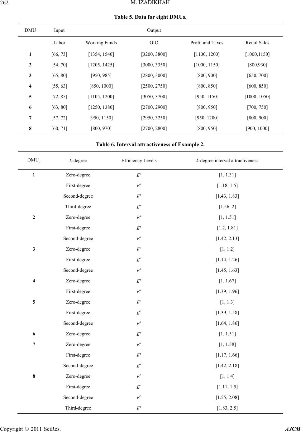

M. IZADIKHAH 262
Table 5. Data for eight DMUs.
DMU Input Output
Labor Working Funds GIO Profit and Taxes Retail Sales
1 [66, 73] [1354, 1540] [3200, 3800] [1100, 1200] [1000,1150]
2 [54, 70] [1205, 1425] [3000, 3350] [1000, 1150] [800,930]
3 [65, 80] [950, 985] [2800, 3000] [800, 900] [650, 700]
4 [55, 63] [850, 1000] [2500, 2750] [800, 850] [600, 850]
5 [72, 85] [1105, 1200] [3050, 3700] [950, 1150] [1000, 1050]
6 [63, 80] [1250, 1380] [2700, 2900] [800, 950] [700, 750]
7 [57, 72] [950, 1150] [2950, 3250] [950, 1200] [800, 900]
8 [60, 71] [800, 970] [2700, 2800] [800, 950] [900, 1000]
Table 6. Interval attractiveness of Example 2.
DMUj k-degree Efficiency Levels k-degree interval attractiveness
1 Zero-degree 3
E [1, 1.31]
First-degree 4
E [1.18, 1.5]
Second-degree 5
E [1.43, 1.83]
Third-degree 6
E [1.56, 2]
2 Zero-degree 4
E [1, 1.51]
First-degree 5
E [1.2, 1.81]
Second-degree 6
E [1.42, 2.13]
3 Zero-degree 4
E [1, 1.2]
First-degree 5
E [1.14, 1.26]
Second-degree 6
E [1.45, 1.63]
4 Zero-degree 5
E [1, 1.67]
First-degree 6
E [1.39, 1.96]
5 Zero-degree 4
E [1, 1.3]
First-degree 5
E [1.39, 1.58]
Second-degree 6
E [1.64, 1.86]
6 Zero-degree 6
E [1, 1.51]
7 Zero-degree 4
E [1, 1.58]
First-degree 5
E [1.17, 1.66]
Second-degree 6
E [1.42, 2.18]
8 Zero-degree 3
E [1, 1.4]
First-degree 4
E [1.11, 1.5]
Second-degree 5
E [1.55, 2.08]
Third-degree 6
E [1.83, 2.5]

M. IZADIKHAH 263
ment. By the same manner one can use the proposed
procedure to calculate interval progress for each DMU.
6. References
[1] A. Charnes, W. W. Cooper and E. Rhodes, “Measuri ng the
Efficiency of Decision Making Units,” European Journal
of Operational Research, Vol. 2, No. 6, 1978, pp. 429-
444. doi:10.1016/0377-2217(78)90138-8
[2] H. Morita, K. Hirokawa an d J. Zhu, “A Slack-Based Mea-
sure of Efficiency in Context Dependent Data Envelop-
ment Analysis,” Omega, Vol. 33, No. 4, 2005, pp. 357-
362. doi:10.1016/j.omega.2004.06.001
[3] L. M. Seiford and J. Zhu, “Context-Dependent Data En-
velopment Analysis: Measuring Attractiveness and Pro-
gress,” Omega, Vol. 31, No. 5, 2003, pp. 397-408.
doi:10.1016/S0305-0483(03)00080-X
[4] J. Zhu, “Quantitative Models for Performance Evaluation
and Benchmarking-Data Envelopment Analysis with Spread-
sheets and DEA Excel Solver,” Kluwer, Boston, 2002.
[5] W. W. Cooper, K. S. Park and G. Yu, “IDEA and AR-
IDEA: Models for Dealing with Imprecise Data in DEA,”
Management Science, Vol. 45, No. 4, 1999, pp. 597-607.
doi:10.1287/mnsc.45.4.597
[6] S. H. Kim, C. G. Park and K. S. Park, “An Application of
Data Envelopment Analysis in Telephone Offices Evalu-
ation with Partial Data,” Computers and Operations Re-
search, Vol. 26, No. 1, 1999, pp. 59-72.
doi:10.1016/S0305-0548(98)00041-0
[7] W. D. Cook, M. Kress and L. Seiford, “Data Envelopment
Analysis in the Presence of Both Quantitative and Quali-
tative Factors,” Journal of the Operational Research So-
ciety, Vol. 47, No. 7, 1996, pp. 945-953.
[8] W. D. Cook, M. Kress and L. Seiford, “On the Use of
Ordinal Data in Data Envelopment Analysis,” Journal of
the Operational Research Society, Vol. 44, No. 2, 1993,
pp. 133-140.
[9] W. D. Cook, J. Doyle, R. Green and M. Kress, “Multiple
Criteria Modeling and Ordinal Data: Evaluation in Terms
of Subset of Criteria,” European Journal of Operational
Research, Vol. 98, No. 3, 1997, pp. 602-609.
doi:10.1016/S0377-2217(96)00069-0
[10] J. Sarkis and S. Talluri, “A Decision Model for Evalua-
tion of Flexible Manufacturing Systems in the Presence
of Both Cardinal and Ordinal Factors,” International
Journal of Production Research, Vol. 37, No. 13, 1999,
pp. 2927-2938. doi:10.1080/002075499190356
[11] D. K. Despotis and Y. G. Smirlis, “Data Envelopment Ana-
lysis with Imprecise Data,” European Journal of Opera-
tional Research, Vol. 140, No. 1, 2002, pp. 24-36.
doi:10.1016/S0377-2217(01)00200-4
[12] G. R. Jahanshahloo, F. Hosse inzadeh Lotfi and M. Moradi,
“Sensitivity and Stability Analysis in DEA with interval
Data,” Applied Mathematics and Computation, Vol. 156,
No. 2, 2004, pp. 463-477. doi:10.1016/j.amc.2003.08.005
[13] M. Izadikhah and F. Hosseinzadeh Lotfi, “Sensitivity Ana-
lysis of Units with Interval Data in DEA,” International
Mathematical Forum, No. 2, Vol. 42, 2007, pp. 2083-2097.
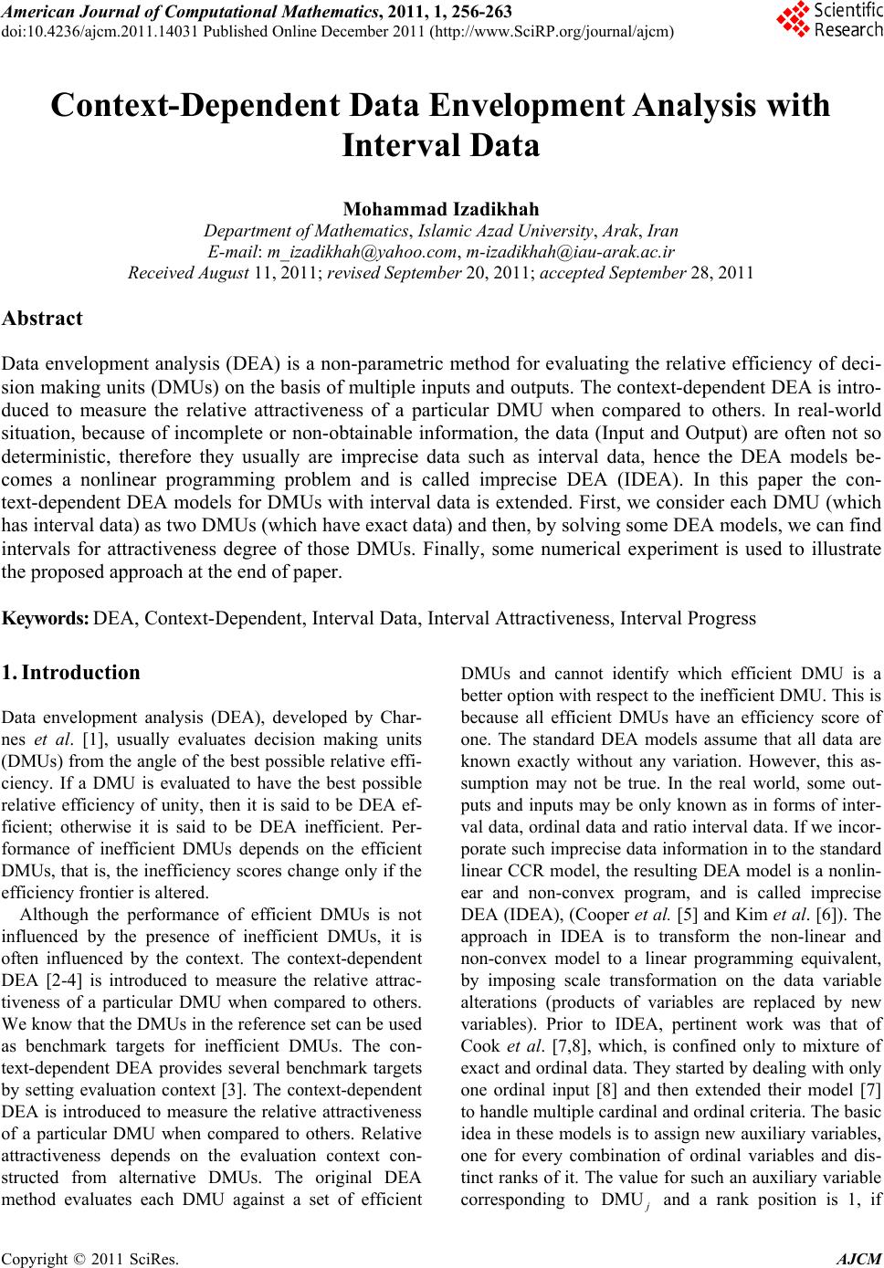