American Journal of Computational Mathematics, 2011, 1, 252-255
doi:10.4236/ajcm.2011.14030 Published Online December 2011 (http://www.SciRP.org/journal/ajcm)
A New Preconditioner with Two Variable Relaxation
Parameters for Saddle Point Linear Systems with Highly
Singular (1,1) Blocks
Yuping Zeng, Chenliang Li
School of Mathematics and Computing Science, Guilin University of Electronic Technology, Guilin, China
Received July 24, 2011; revised August 26, 2011; accepted September 6, 2011
Abstract
In this paper, we provide new preconditioner for saddle point linear systems with (1,1) blocks that have a
high nullity. The preconditioner is block triangular diagonal with two variable relaxation paremeters and it is
extension of results in [1] and [2]. Theoretical analysis shows that all eigenvalues of preconditioned matrix is
strongly clustered. Finally, numerical tests confirm our analysis.
Keywords: Saddle Point Linear Systems, Block Triangular Preconditioner, Krylov Subspace Methods
1. Introduction
Consider the following saddle point linear system
,
0
Tuf
FB
A
x
pg
B






 b (1)
where nn
F
R 
n
is symmetric and positive semidefinite
with nullity r, has full row rank,

mn
BR mn



f
R and n
g
R, u and p are unknown. Note that
the assumption that A is nonsingular, i.e., the system (1)
has a unique solution implies that null(F)/null(B) = 0,
which we use in our analysis below. Saddle point linear
systems of form (1) can arise, for example, from con-
straint optimization [3], mixed nite element formulation
for the stokes problem [4], and discrete time harmonic
Maxwell equations in mixed form [5].
There has many techniques for solving Saddle point
linear systems of form (1), see [6] for a comprehensive
survey. However, when F is singular, it cannot be in-
verted and the Schur complement does not exist. In this
case, one possible way of dealing with system is by
augmentation [7]. Another way we can refer to [8] where
Grief and SchÄotzau exploited a preconditioning techni-
que for solving time-harmonic Maxwell equations in
mixed form.
Recently, Rees and Grief [2] extend the work by Grief
and SchÄotzau [8] to interior point methods for optimi-
zation problems. The preconditioner has attractive proper-
ty of improved eigenvalue clustering with ill-conditioned
the (1,1) block of saddle point systems. Based on the
basic of above work, Huang etc. costructed two block
triangular preconditioners for solving saddle point sys-
tems (1) [1].
In this paper we are devoted to give new block trian-
gular preconditioner for solving saddle point systems of
(1) with an ill-conditioned (1,1) blocks. The precondi-
tioner is involving two parameters, and they are exten-
sion of recent work in Grief and SchÄotzau [8], Rees and
Grief [2], and Cheng etc. [1].
2. New Preconditioner and Spectral Analysis
Rees and Grief [9] provided the following preconditioner
for the symmetric saddle point systems (1)
1
,
0
TT
FBWBtB
MW





where t is a scalar and is symmetric positive
weight matrix.
mm
WR


Recently, Huang etc. [6] established the following pre-
conditioners for the saddle point systems:

11,
0
TT
t
FBWBtB
MtW





where 0t

is a parameter and

1
ˆ,
1
0
TT
t
FtBWB tB
MtW
t









Y. P. ZENG ET AL.253

where . 10t
In this section, we introduce the following precondi-
tioner involving two parameters:

1
,
1,
0
TT
FBWB B
MW








(2)
for the saddle point systems (1), where 0

 and
0

. We note that when the parameter 1


, and
t

,
M


reduce to t
M
; when t

 and 1t
t


,
M


reduce to t
M
.
Theorem 2.1. The matrix 1
M
A

 has two distinct ei-
genvalues, given by
11

 and 21

  ,
with the algebraic multiplicities n and r, respectively.
The remaining m − r eigenvalues satisfy the relation

,
1

   (3)
where

are positive generalized eigenvalues of
1, T
B WBuFu 
 (4)
Let 1i be a basis of the null space of F, 1i

r
i
x

nm
i
z


be a basis of the null space of B, and 1i a set of
linearly independent vectors that complete null(F)
null(B) to a basis of Rn, Then the r vectors

nm
i
y

1
1
;
ii
x
WBx








, the n − m vectors , and the m − r
vectors

;0
i
z
1
1
,
i
yWBy





i


are linearly independent eigenvec-
tors associated with 1

, and the r vectors

1
;
i

i
x
WBx 

 are eigenvectors associated with
1



 .
Proof: Suppose that

is an eigenvalue of 1
ˆ
M
A

,
whose eigenvector is . Then the correspond-

T
u
p
,T
TT
up
ing eigenvalue problem is

11.
00
TT
u
FBF BWBuB
p
BW



 

 

 
 
 
 
From the second row we can obtain 1
1
pWB


u .
By substituting it into the first row we have

1
1
10
T
FuB WBu  









.
(5)
If 1


;uW
, then (5) is satisfied for any , and
hence is an eigenvector of
n
uR
1

1Bu 

M
A

.
If null(F), then from (5) we obtain u

1
1
10
T
BW Bu 


 .




From which it follows that 1
1
;uWBu





and


1
;uWBu 

 are eigenvectors associated 1


and
1



.
Next, suppose 1


and 1

  . We divide (5)
by




11

  , which yields (3), with u defined in
(4).
Now we can find a specific set of linearly independent
eigenvectors for 1


and 1

  . Since null(F) ∩
null(B) = 0, the vectors

1i and 1i
r
i
x

nm
i
z

 defined
above are linearly independent and form a subspace of
n
R
of dimension n − m + r. Let

1
ii complete this
set to a basis of Rn . It follows that ii
nm
,
y

11
x
WBx

 ,


,0
i
z, and


By
11
yW 

,
ii
are eigenvectors associated
with 1


. The r vectors

1
i

,i
x
WB
x
  are igenvec-
tors associated with 1



.
When the parameters satisfy 11

 , we can obtain
the following corollary from Theorem 2.1.
Corollary 2.2. Let 11



. Then the matrix 1
M
A


has one eigenvalue which given by 1

 with algebraic
multiplicity n + r. The remaining m − r eigenvalues sat-
isfy the relation

1, 


where µ are positive generalized eigenvalues of
1T
B WBuFu 
.
Theorem 2.3. The matrix 1
M
A

 has two distinct ei-
genvalues, given by
11


and 21

  ,
with the algebraic multiplicities n and r, respectively.
The remaining m − r eigenvalues lie in the interval




0,10 ,or1,00  


 
.
Proof: From Theorem 2.1 we obtain that the matrix
1
M
A

 has two distinct eigenvalues, given by
11


and 21

  ,
with the algebraic multiplicities n and r, respectively.
Taking inner product of (5) with u, we can obtain that
the remaining m − r eigenvalues satisfy

1
1
,
,,
T
T
BW Buu
F
uuBW Buu





, (6)
where ,

 denotes the standard Euclidean inner prod-
uct, u

null(F) and u

null(B). By (6), we have that
the remaining m − r eigenvalues lie in interval

Y. P. ZENG ET AL. 254


 
0,10 ,or1,00    .
When the parameters satisfy 11

 , we can obtain
the following corollary from Theorem 2.3.
Corollary 2.4. Let 11

 . Then the matrix 1
M
A


has one eigenvalue which given by λ = 1 with algebraic
multiplicity n + r. The remaining m − r eigenvalues lie in
the interval (0, 1).
3. Numerical Experiments
We consider the following finite element discretization
of the time-harmonic Maxwell equations (k2 = 0) [5,8].
The following two-dimensional Model problem is con-
sidered: find u and p that satisfy
in
0in
0on
0on
upf
u
u
p
 
 
 

n

(7)
Here is a simply connected polyhedron do-
main with a connected boundary ∂Ω, and ~n denotes the
outward unit normal on ∂Ω. The datum
2
R
f
is a given
source (not necessarily divergence free). Using the low-
est order N’ed’elec elements of first kind [9,10] for the
approximation of the vector field and standard nodal
elements for multiplier yields the following saddle-point
linear system
.
0
0
Tug
FB
A
x
p
B






 b
Experiments were done in a square domain (0 ≤ x ≤ 1;
0 ≤ y ≤ 1). And we set the right-hand side function so
that the exact solution is given by
  
,1,1
T
uxyyyxx .
In our numerical experiments the matrix W in the
augmentation block preconditioner is taken as W = I.
We consider three meshes with different values of n
and m in Table 1. Table 2 shows iteration counts for
different η and meshes, applying BiCGSTAB of
block-triangular preconditioner, and 11

 . We ob-
Table 1. Values of n and m and size of the linear systems for
three meshes.
h n m n + m
1
8 176 49 225
1
16 225 736 961
1
32 961 3008 3969
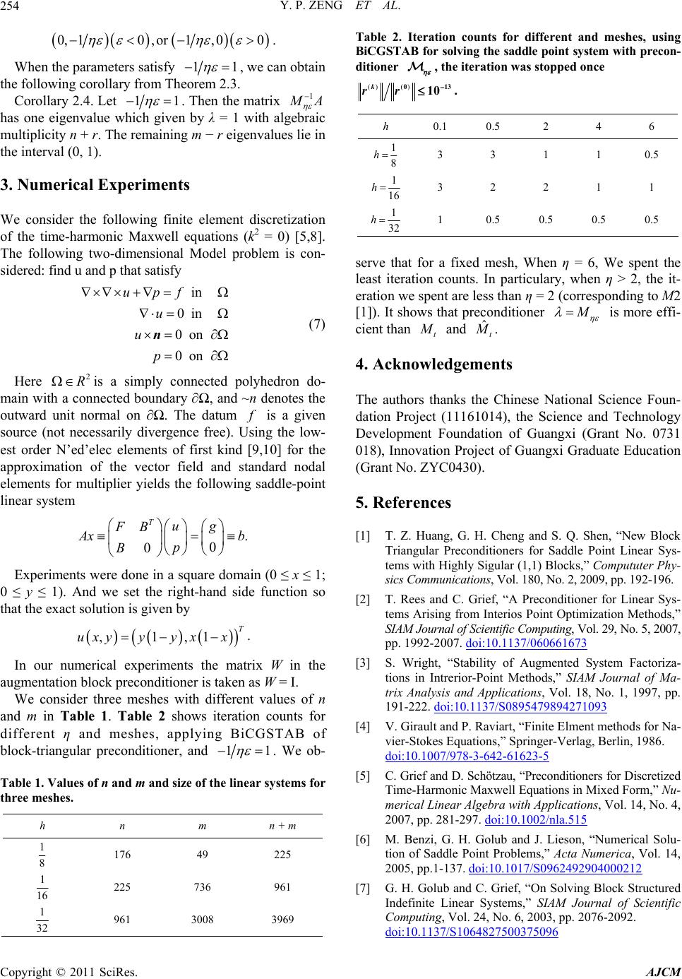
Table 2. Iteration counts for different and meshes, using
BiCGSTAB for solving the saddle point system with precon-
ditioner


, the iteration was stopped once
() 013k
rr
()10

.
h 0.1 0.5 2 4 6
1
8
h

3 3 1 1 0.5
1
16
h3 2 2 1 1
1
32
h1 0.5 0.5 0.5 0.5
serve that for a fixed mesh, When η = 6, We spent the
least iteration counts. In particulary, when η > 2, the it-
eration we spent are less than η = 2 (corresponding to M2
[1]). It shows that preconditioner
M



 is more effi-
cient than t
M
and ˆt
M
.
4. Acknowledgements
The authors thanks the Chinese National Science Foun-
dation Project (11161014), the Science and Technology
Development Foundation of Guangxi (Grant No. 0731
018), Innovation Project of Guangxi Graduate Education
(Grant No. ZYC0430).
5. References
[1] T. Z. Huang, G. H. Cheng and S. Q. Shen, “New Block
Triangular Preconditioners for Saddle Point Linear Sys-
tems with Highly Sigular (1,1) Blocks,” Compututer Phy-
sics Communications, Vol. 180, No. 2, 2009, pp. 192-196.
[2] T. Rees and C. Grief, “A Preconditioner for Linear Sys-
tems Arising from Interios Point Optimization Methods,”
SIAM Journal of Scientific Computing, Vol. 29, No. 5, 2007,
pp. 1992-2007. doi:10.1137/060661673
[3] S. Wright, “Stability of Augmented System Factoriza-
tions in Intrerior-Point Methods,” SIAM Journal of Ma-
trix Analysis and Applications, Vol. 18, No. 1, 1997, pp.
191-222. doi:10.1137/S0895479894271093
[4] V. Girault and P. Raviart, “Finite Elment methods for Na-
vier-Stokes Equations,” Springer-Verlag, Berlin, 1986.
doi:10.1007/978-3-642-61623-5
[5] C. Grief and D. Schötzau, “Preconditioners for Discretized
Time-Harmonic Maxwell Equations in Mixed Form,” Nu-
merical Linear Algebra with Applications, Vol. 14, No. 4,
2007, pp. 281-297. doi:10.1002/nla.515
[6] M. Benzi, G. H. Golub and J. Lieson, “Numerical Solu-
tion of Saddle Point Problems,” Acta Numerica, Vol. 14,
2005, pp.1-137. doi:10.1017/S0962492904000212
[7] G. H. Golub and C. Grief, “On Solving Block Structured
Indefinite Linear Systems,” SIAM Journal of Scientific
Computing, Vol. 24, No. 6, 2003, pp. 2076-2092.
doi:10.1137/S1064827500375096

Y. P. ZENG ET AL. 255
[8] C. Grief and D. Schötzau, “Preconditioners for Saddle
Point Linear Systems with Highly Singular (1,1) Blocks,”
Electronic Transactions on Numerical Analysis, Vol. 22,
2006, pp. 114-121.
[9] P. Monk, “Finite Elements for Maxwell’s Quations,” Ox-
frod University Press, New York, 2003.
[10] J. C. Nédélec, “A New Family of Mixed Finite Elements
in ℝ3,” Numerische Mathematik, Vol. 50, No. 1, 1986, pp.
57-81. doi:10.1007/BF01389668