American Journal of Computational Mathematics, 2011, 1, 226-234
doi:10.4236/ajcm.2011.14026 Published Online December 2011 (http://www.SciRP.org/journal/ajcm)
Solution of the Generalized Abel Integral Equation by
Using Almost Bernstein Operational Matrix
Sandeep Dixit1, Rajesh K. Pandey2, Sunil Kumar1, Om P. Singh1
1Department of Applied Mathematics, Institute of Technology, Banaras Hindu University, Varanasi, India
2PDPM Indian Institute of Information Technology, Design and Manufacturing, Jabalpur, India
Received June 12, 2011; revised July 5, 2011; accepted July 15, 2011
Abstract
A direct almost Bernstein operational matrix of integration is used to propose a stable algorithm for numeri-
cal inversion of the generalized Abel integral equation. The applicability of the earlier proposed methods was
restricted to the numerical inversion of a part of the generalized Abel integral equation. The method is quite
accurate and stable as illustrated by applying it to intensity data with and without random noise to invert and
compare it with the known analytical inverse. Thus it is a good method for applying to experimental intensi-
ties distorted by noise.
Keywords: Abel Inversion, Bernstein Polynomials, Almost Bernstein Operational Matrix of Integration,
Noise Resistance
1. Introduction
Abel’s integral equation [1] occurs in many branches of
science. Usually, physical quantities accessible to meas-
urement are quite often related to physically important but
experimentally inaccessible ones by Abel’s integral equa-
tion. Some of the examples are: microscopy [2], seis-
mology [3,4], radio astronomy [5], satellite photometry
of airglows [6], electron emission [7], atomic scattering
[8], radar ranging [9], and optical fiber evaluation [10-12].
But it is most extensively used in flame and plasma di-
agnostics [13-15] and X-ray radiography [16-19].
Recently, Chakrabarti [20] employed a direct function
theoretic method to determine the closed form solution
of the following generalized Abel integral equation
 
    
 
dd
,
01, ,
x
x
tt tt
axbxf x
xt tx
x








 
 (1)
where the coefficients and do not vanish
simultaneously.

ax

bx
Earlier the generalized Abel equation (1) was exam-
ined in Gakhov’s book [21], under the special assump-
tions that the coefficients and satisfy Hol-
der’s condition in

ax

bx


,

 , whereas the forcing term

f
x and the unknown function

x
 belong to those
class of functions which admit representations of the
form
 
 


*
*
1
,
0,
fxxxf x
x
xxx








 









(2)
where


*
f
x possesses a Holder continuous derivative
in


,

 and


*
x
 satisfies Holder’s condition in


,

 .
The method of Gakhov’s has a particular disadvantage
in the sense that while solving a singular equation that
involves integrals only with weak singularity of the type

0tx




1



1
tx
, occurrence of strongly singular
integrals involving Cauchy type singularities of the type

 has to be permitted [20,21]. Chakrabarti [20]
obtained the solution involving only weakly singular
integrals of the Abel type and thus Cauchy type singular
integrals were avoided. But the numerical inversion is
still needed for its application in physical models since
the experimental data for the intensity 
f
x is avail-
able only at a discrete set of points and it may also be
distorted by noise.
The aim of the present paper is to propose a new stable
algorithm for the numerical inversion of Abel’s integral
equation (1), based on the newly constructed almost
Bernstein operational matrices of integration. Numerical
examples are given to illustrate the accuracy and stability

S. DIXIT ET AL.227
of the proposed algorithm.
2. The Bernstein Polynomials
A Bernstein polynomial, named after Sergei Natanovich
Bernstein, is a polynomial in the Bernstein form that is a
linear combination of Bernstein basis polynomials.
The Bernstein basis polynomials of degree are de-
fined by
n
,()(1) ,0,1,2,,
ini
in
n
Btt tin
i





. (3)
There are degree Bernstein basis polyno-
mials forming a basis for the linear space n consisting
of all polynomials of degree less than or equal to in
R[x]—the ring of polynomials over the field R. For
mathematical convenience, we usually set

1th nnVn
0
,in
B

if
or . 0iin
Any polynomial in may be written as

Bx n V
 
,
0
n
iin
i
BxB x 

. (4)
Then is called a polynomial in Bernstein form
or Bernstein polynomial of degree . The coefficients
i

Bx n

are called Bernstein or Bezier coefficients. But sev-
eral mathematicians call Bernstein basis polynomials
as the Bernstein polynomials. We will follow
this convention as well. These polynomials have the fol-
lowing properties:

x
,in
B
1)

,0
0
in i
B

 and


,1 in in
B

, where

is the
Kronecker delta function.
2) has one root, each of multiplicity and
, at and respectively.

,in
Bt
i0ti n1t
3) for

,0 in
Bt


0,1t

1Bt
and

,,inn in
B


t.
4) For , ,in has a unique local maximum in 0iB


0,1 at tin and the maximum value

ni
in n
innii




.
5) The Bernstein polynomials form a partition of unity
i.e. .

,
0
1
n
in
i
Bt



Using Gram-Schmidt orthonormalization process on
,in, we obtain a class of orthonormal polynomials. We
call them orthonormal Bernstein polynomials of order
and denote them by .
Bn
01
,,,
nn nn
bb b
3. Function Approximation
A function


20,1fL may be written as
 
0
lim
n
in in
ni
f
tcb
 

where, ,
in in
ccb and , is the standard inner prod-
uct on


20,1L.
If the series (5) is truncated at , then we have nm

0
mT
im im
i
f
cb CBt


, (6)
where, and
C


Bt are matrices given by

11m
T

01
,,, ,
mm mm
Ccc c

(7)
and

01
,,, T
mm mm
Btbtbtbt




. (8)
4. Solution of Generalized Abel Integral
Equation
In this section we solve generalized Abel integral equa-
tion by orthonormal Bernstein polynomials.
Using Equation (8), we approximate


x
 and


f
x as



 
,,
TT
x
CBxf xFBx  
  (9)
where the matrix
F
is known. Then from equation (1)
and (9) we have



  
 
dd
TT
xT
x
CBt tCBt t
ax bxFBx
tx tx





 (10)
From Equation (8) and from the derived formulae,

1
1
21
d(1 )
(1 )1, ;2;,
(2 )
xn
nn
tt nx
xt
xFn n
nx








 


 







(11)
 

1
1
21
d1
1,1;;
()
n
x
nn
tt n
tx
xx
Fnn
n









 


 




 


,
(12)
it is obvious that


    
d,d
x
x
Bt Bt
tPBx tQx
xt tx






, (13)
where and are
PQ

 
1mm1

 matrices, which
we call as almost Bernstein operational matrix of inte-
gration for Abel integral equation with generalized ker-
nel.
Substituting (13) in (10), we get
t, (5)
 

1
TT
CFaxPbxQ



(14)

S. DIXIT ET AL. 228
Hence, the approximate solution for general-
ized Abel integral equation (1) is obtained by putting the
value of from (14) in (9).

t 

T
C
and compute the corresponding errors and level
them as

Et






1,2,3,4EtEtEtEt
1

respectively. Then
a noise term

is introduced in forcing term


f
x
and for 1000, 500N

the corresponding errors


5Et,






7,8EtEt

6,Et and
 


12E t9,10EtE,11E t,t,
are computed for the four chosen values of

as men-
tioned above. In all the figures some of the error terms


j
Et are multiplied by 10 or some power of 10 for
suitable scaling. Also we tabulated the approximate and
exact solutions through Tables 1-4 for the four examples
given below for various values of .
t
5. Illustrative Examples
The following examples are solved with and without
noise terms to illustrate the efficiency and stability of our
method. Note that in all the examples to follow, the se-
ries (5) is truncated at level 6m

and hence the almost
operational matrix in (13) is of order .
77Example 1. Consider the generalized Abel integral
equation with




1ax bx

 and
The accuracy of the proposed algorithm is demon-
strated by calculating the parameters of absolute error
and average deviation

i
t  

also known as root
mean square error (RMS). They are calculated using the
following equations:
 
ii
Ettt  
i
and
 
12 12
22
11
2
11
,
NN
Nii
ii
tt t
NN
 










i



(15)


 

612
21
10395 π11 secπ
15
65 2
1313 11
,,, ,
222
fx
xxxx
Fx







 




 
 
 
 

(16)
where 21
F
 is the regularized hypergeometric function.
This has the exact solution

11 2
tt  .
where is the approximate solution calculated at
point i and is the exact solution at the corre-
sponding point. Note that

i
t 

t

i
t

, henceforth, denoted by
N

(for computational convenience) is the discrete
-norm of the absolute error
2
l


denoted by
Figure 1 illustrates the effect of the absolute errors
without noise for different values of

, whereas Fig-
ures 2 and 3 show the absolute errors with noise term
1

added to the forcing term

f
x for = 1000,
500 respectively. Table 1 compares the approximate and
exact values of Example 1.
N
.

2
Note that the calculation of
N

is performed by tak-
ing = 1000, 500 in Equation (15). In all the exam-
ples, the exact and noisy profiles are denoted by
N


f
x
and

f
x

, respectively, where

f
x

is obtained by
adding a noise

to

f
x such that

fx

x
Example 2. Consider the generalized Abel integral
equation with




1ax bx

 and
  




22 2
4
2
2
21314 3
4321
6
12 7
23
xxx
fx
x
xx

















, (17)
ii

i
f

  , where ,1,,,1
i
x
ih i NNh 
is the uniform random variable with values in and i

[–1, 1] such that
 
1
max ii
iN fxfx




.
The following examples are solved with and without
noise to illustrate the efficiency and stability of our
method by choosing two different values of the noises
j

as 01 0, .
N

 In all the examples to follow, we
take four different values of

as 1/10, 1/4, 1/2, 3/4
having the exact solution .

3
ttt  
Figure 4 illustrates the effect of the absolute errors
Table 1. Approximate and exact solution of Example 1.
t 0.0 0.2 0.4 0.6 0.8 1.0

t  0 0.00014 0.00648 0.06023 0.29309 1.0000

t  at 110   0.00013 0.00018 0.00647 0.06020 0.29308 1.00025

t  at 14   0.00001 0.00016 0.00646 0.06020 0.29311 1.00003

t  at 12   –0.00004 0.00013 0.00646 0.06024 0.29309 1.00004

t  at 34   –0.00004 0.00011 0.00646 0.06023 0.29308 1.00001

S. DIXIT ET AL.229
Table 2. Approximate and exact solution of Example 2.
t 0.0 0.2 0.4 0.6 0.8 1.0

t  0 0.19200 0.33600 0.38400 0.28800 0.0000

t  at 110  –0.00001 0.19199 0.33599 0.38400 0.28798 –0.000005

t  at 14  –0.00001 0.19200 0.33601 0.38400 0.28801 –0.000033

t  at 12  –0.00004 0.19200 0.33600 0.38400 0.28800 –0.000038

t  at 34  –0.00037 0.19195 0.33601 0.38396 0.28800 0.00014
Table 3. Approximate and exact solutions of Example 3.
t 0.0 0.2 0.4 0.6 0.8 1.0

t  1 1.2214 1.49182 1.82212 2.22554 2.71828

t  at 110   1.0002 1.22145 1.49183 1.82210 2.22558 2.71828

t  at 14   1.00004 1.22140 1.49182 1.82214 2.22550 2.71853

t  at 12   1.00012 1.22140 1.49183 1.82212 2.22556 2.71831

t  at 34   1.00156 1.22116 1.49180 1.82190 2.22557 2.71868
Table 4. Approximate and exact solutions of Example 4.
t 0.0 0.2 0.4 0.6 0.8 1.0

t  0.0 0.03959 0.07306 0.10206 0.12764 0.15051

t  at 110   0.00017 0.03960 0.07305 0.10204 0.12762 0.15073

t  at 14   0.00008 0.03955 0.07307 0.10208 0.12762 0.15056

t  at 12   –0.00006 0.03960 0.07306 0.10206 0.12764 0.15052

t  at 34   0.00007 0.03958 0.07306 0.10205 0.12764 0.15055
00.20.40.60.81
0
1.5 10 4
310 4
4.5 10 4
610 4
E1 t()
10 E2t()
10 E3t()
10 E4t()
t
6×10
–4
4.5×10
–4
3×10
–4
1.5×10
–4
Figure 1. Comparison of absolute errors, Example 1.
without noise for different values of

, whereas Fig-
ures 5 and 6 show the absolute errors with noise term
1

added to the forcing term


f
x for =1000,
500 respectively. Table 2 compares the approximate and
exact values of Example 2.
N
Example 3. Consider the generalized Abel integral
equation with and
 
1axbx





 

 
  
111,11
11,
x
x
fx exxx
ex





 
 (18)
This has the exact solution .

t
te  
Figure 7 illustrates the effect of the absolute errors
without noise for different values of

, whereas Fig-
res 8 and 9 show the absolute errors with noise term u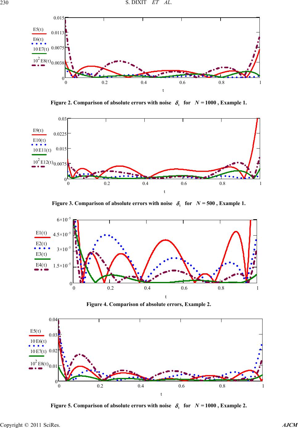

S. DIXIT ET AL. 230
00.2 0.40.60.81
0
0.0038
0.0075
0.0113
0.015
E5 t()
E6 t()
10 E7t()
102E8 t()
t
Figure 2. Comparison of absolute errors with noise 1

for , Example 1. = 1000N
00.20.4 0.6 0.81
0
0.0075
0.015
0.0225
0.03
E9 t()
E10 t()
10 E11t()
102E12 t()
t
Figure 3. Comparison of absolute errors with noise 1

for , Example 1. = 500N
00.2 0.4 0.6 0.81
0
1.5 10 5
310 5
4.5 10 5
610 5
E1 t()
E2 t()
E3 t()
E4 t()
t
6×10
–5
4.5×10
–5
3×10
–5
1.5×10
–5
Figure 4. Comparison of absolute errors, Example 2.
00.20.40.6 0.81
0
0.01
0.02
0.03
0.04
E5 t()
10 E6t()
10 E7t()
102E8 t()
t
Figure 5. Comparison of absolute errors with noise 1

for , Example 2. = 1000N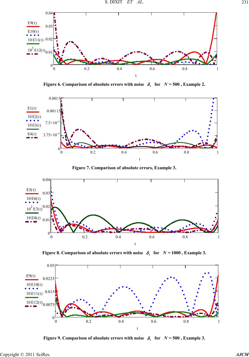

S. DIXIT ET AL.231
00.2 0.40.6 0.81
0
0.01
0.02
0.03
0.04
E9 t()
E10 t()
10 E11t()
102E12 t()
t
Figure 6. Comparison of absolute errors with noise 1

for , Example 2. = 500N
00.20.40.60.8
0
3.75 10
1
4
7.5 104
0.00113
0.0015
E1 t()
10 E2t()
10 E3t()
E4 t()
t
7.5×10
–4
3.75×10
–4
Figure 7. Comparison of absolute errors, Example 3.
00.2 0.40.6 0.81
0
0.01
0.02
0.03
0.04
E5 t()
10 E6t()
102E7 t()
10 E8t()
t
Figure 8. Comparison of absolute errors with noise 1

for , Example 3. = 1000N
00.2 0.4 0.6 0.81
0
0.0075
0.015
0.0225
0.03
E9 t()
10 E10t()
10 E11t()
10 E12t()
t
Figure 9. Comparison of absolute errors with noise 1

for , Example 3. = 500N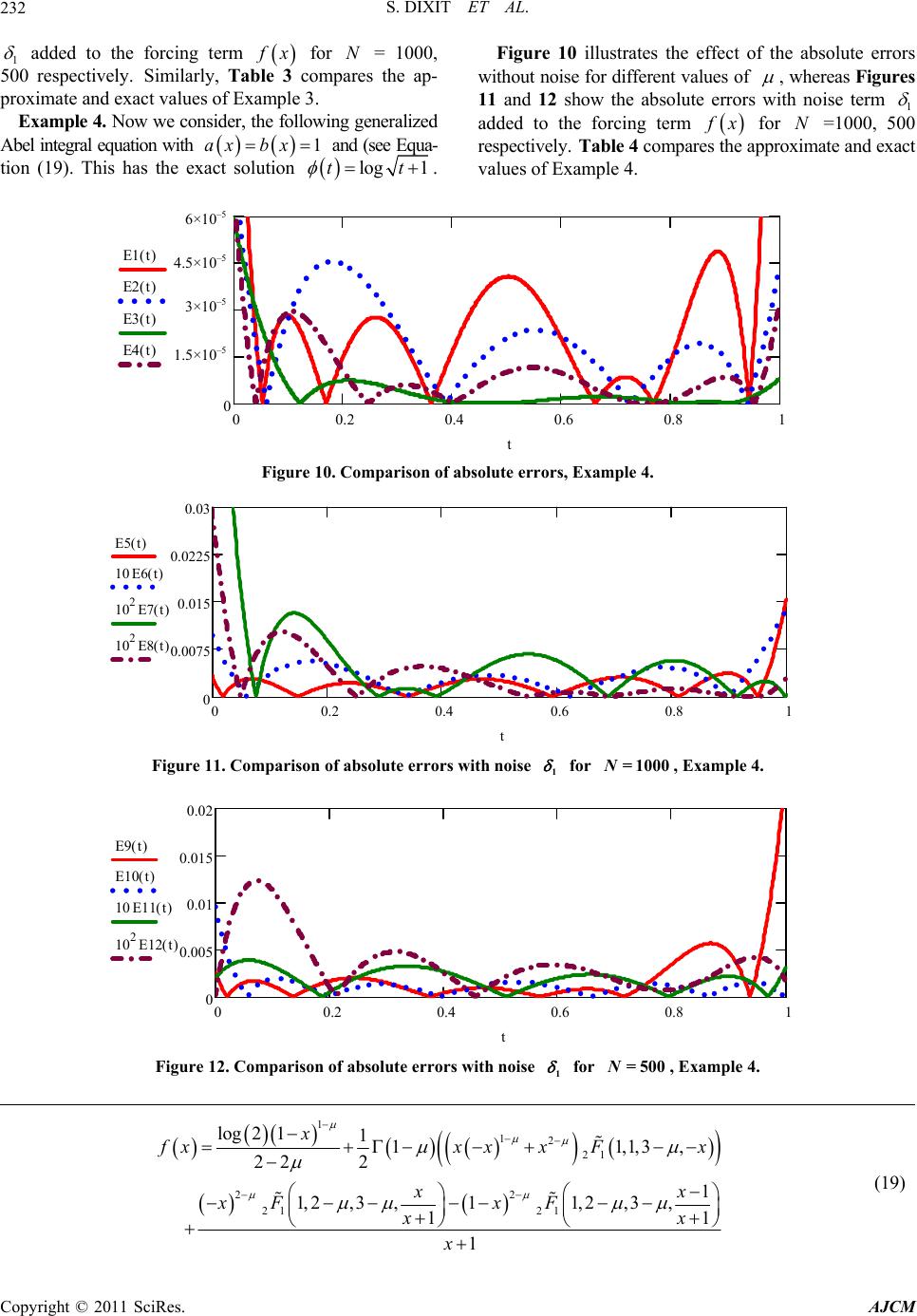

S. DIXIT ET AL. 232
1

added to the forcing term

f
x for = 1000,
500 respectively. Similarly, Table 3 compares the ap-
proximate and exact values of Example 3.
NFigure 10 illustrates the effect of the absolute errors
without noise for different values of

, whereas Figures
11 and 12 show the absolute errors with noise term 1

added to the forcing term

f
x for =1000, 500
respectively. Table 4 compares the approximate and exact
values of Example 4.
N
Example 4. Now we consider, the following generalized
Abel integral equation with and (see Equa-
tion (19). This has the exact solution
 
1axbx


log 1tt  
.
00.2 0.4 0.6 0.81
0
1.5 10 5
310 5
4.5 10 5
610 5
E1 t()
E2 t()
E3 t()
E4 t()
t
6×10
–5
4.5×10
–5
3×10
–5
1.5×10
–5
Figure 10. Comparison of absolute errors, Example 4.
00.2 0.40.6 0.81
0
0.0075
0.015
0.0225
0.03
E5 t()
10 E6t()
102E7t()
102E8t()
t
Figure 11. Comparison of absolute errors with noise 1

for , Example 4. = 1000N
00.2 0.4 0.6 0.81
0
0.005
0.01
0.015
0.02
E9 t()
E10 t()
10 E11t()
102E12 t()
t
Figure 12. Comparison of absolute errors with noise 1

for , Example 4. = 500N
  



 
1
12
21
22
21 21
log 21111,
22 2
1
1, 2, 3,11,2, 3,
11
1
x1,3,
f
xxxxF
xx
xF xF
xx
x





 





x


 
 







(19)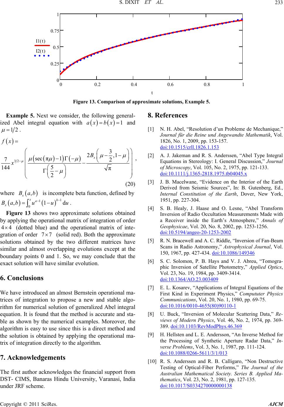

S. DIXIT ET AL.233
00.2 0.4 0.6 0.81
0
0.25
0.5
0.75
1
I1 t()
I2 t()
t
Figure 13. Comparison of approximate solutions, Example 5.
Example 5. Next we consider, the following general-
ized Abel integral equation with and
 
1axbx
12

.


  
32
3
2,1
sec π1
72
5
144 π
2
x
fx
B
x


 








 


 











d
,
(20)
where is incomplete beta function, defined by

,
x
Bab
1
xa
 
1
0
,1
b
x
Babuu u


.
Figure 13 shows two approximate solutions obtained
by applying the operational matrix of integration of order
(dotted blue) and the operational matrix of inte-
gration of order (solid red). Both the approximate
solutions obtained by the two different matrices have
similar and almost overlapping evolutions except at the
boundary points 0 and 1. So, we may conclude that the
exact solution will have similar evolution.
44
77
6. Conclusions
We have introduced an almost Bernstein operational ma-
trices of integration to propose a new and stable algo-
rithm for numerical solution of generalized Abel integral
equation. It is found that the method is accurate and sta-
ble as shown by the numerical examples. Moreover, the
algorithm is easy to use since this is a direct method and
the solution is obtained by applying the operational ma-
trix of integration directly to the algorithm.
7. Acknowledgements
The first author acknowledges the financial support from
DST- CIMS, Banaras Hindu University, Varanasi, India
under JRF scheme.
8. References
[1] N. H. Abel, “Resolution d’un Probleme de Mechanique,”
Journal für die Reine und Angewandte Mathematik, Vol.
1826, No. 1, 2009, pp. 153-157.
doi:10.1515/crll.1826.1.153
[2] A. J. Jakeman and R. S. Anderssen, “Abel Type Integral
Equations in Stereology: I. General Discussion,” Journal
of Microscopy, Vol. 105, No. 2, 1975, pp. 121-133.
doi:10.1111/j.1365-2818.1975.tb04045.x
[3] J. B. Macelwane, “Evidence on the Interior of the Earth
Derived from Seismic Sources”, In: B. Gutenberg, Ed.,
Internal Constitution of the Earth, Dover, New York,
1951, pp. 227-304.
[4] S. B. Healy, J. Haase and O. Lesne, “Abel Transform
Inversion of Radio Occultation Measurements Made with
a Receiver inside the Earth’s Atmosphere,” Annals of
Geophysicae, Vol. 20, No. 8, 2002, pp. 1253-1256.
doi:10.5194/angeo-20-1253-2002
[5] R. N. Bracewell and A. C. Riddle, “Inversion of Fan-Beam
Scans in Radio Astronomy,” Astrophysical Journal, Vol.
150, 1967, pp. 427-434. doi:10.1086/149346
[6] S. C. Solomon, P. B. Hays and V. J. Abreu, “Tomogra-
phic Inversion of Satellite Photometry,” Applied Optics,
Vol. 23, No. 19, 1984, pp. 3409-3414.
doi:10.1364/AO.23.003409
[7] E. L. Kosarev, “Applications of Integral Equations of the
First Kind in Experiment Physics,” Compututer Physics
Communications, Vol. 20, No. 1, 1980, pp. 69-75.
doi:10.1016/0010-4655(80)90110-1
[8] U. Buck, “Inversion of Molecular Scattering Data,” Re-
views of Modern Physics, Vol. 46, No. 2, 1974, pp. 369-
389. doi:10.1103/RevModPhys.46.369
[9] H. Hellsten and L. E. Andersson, “An Inverse Method for
the Processing of Synthetic Aperture Radar Data,” In-
verse Problems, Vol. 3, No. 1, 1987, pp. 111-124.
doi:10.1088/0266-5611/3/1/013
[10] R. S. Anderssen and R. B. Calligaro, “Non Destructive
Testing of Optical-Fiber Performs,” The Journal of the
Australian Mathematical Society. Series B. Applied Ma-
thematics, Vol. 23, No. 2, 1981, pp. 127-135.
doi:10.1017/S0334270000000138

S. DIXIT ET AL. 234
[11] K. Taketura, “Index Profile Determination of Single-Mode
Fiber by the Phase Contrast Method: A Proposed Tech-
nique,” Applied Optics, Vol. 21, No. 23, 1982, pp. 4260-
4263. doi:10.1364/AO.21.004260
[12] W. J. Glantschnig, “How Accurately Can One Reconstruct
an Index Profile from Transverse Measurement Data,”
Journal of Lightwave Technology, Vol. 3, No. 3, 1985, pp.
678-683. doi:10.1109/JLT.1985.1074221
[13] E. Keren, E. Bar-Ziv, I. Glatt and O. Kafri, “Measurements
of Temperature Distribution of Flames by Moiré Deflec-
tometry,” Applied Optics, Vol. 20, No. 24, 1981, pp. 4263-
4266. doi:10.1364/AO.20.004263
[14] C. J. Tallents, M. D. J. Burgess and B. Luther-Davies,
“The Determination of Electron Density Profiles from Re-
fraction Measurements Obtained Using Holographic In-
terferometry,” Optics Communications, Vol. 44, No. 6,
1983, pp. 384-387. doi:10.1016/0030-4018(83)90222-5
[15] C. Fleurier and J. Chapelle, “Inversion of Abel’s Integral
Equation Application to Plasma Spectroscopy,” Compu-
tuter Physics Communications, Vol. 7, No. 4, 1974, pp.
200-206. doi:10.1016/0010-4655(74)90089-7
[16] K. M. Hanson, “Tomographic Reconstruction of Axially
Symmetric Objects from a Single Radiograph,” Proceed-
ings of SPIE 16th International Conference on High
Speed Photography and Photonics, Vol. 491, 1984, pp.
180-187.
[17] W. J. Glantschnig and A. Holliday, “Mass Fraction Pro-
filing Based on X-Ray Tomography and Its Application
to Characterising Porous Silica Boules,” Applied Optics,
Vol. 26, No. 6, 1987, pp. 983-989.
doi:10.1364/AO.26.000983
[18] A. M. Cormack, “Representation of a Function by Its
Line Integrals with Some Radiological Applications,”
Journal of Applied Physics, Vol. 34, No. 9, 1963, pp.
2722-2727. doi:10.1063/1.1729798
[19] M. Deutsch, A. Notea and D. Pal, “Inversion of Abel’s
Integral Equation and Its Application to NDT by X-Ray
Radiography,” NDT International, Vol. 23, No.1, 1990,
pp. 32-38.
[20] A. Chakrabarti, “Solution of the Generalized Abel Integral
Equation,” Journal of Integral Equation s and Appl ication s,
Vol. 20, No. 1, 2008, pp. 1-11.
doi:10.1216/JIE-2008-20-1-1
[21] F. D. Gakhov, “Boundary Value Problems,” Pergamon
Press, Oxford, 1966.
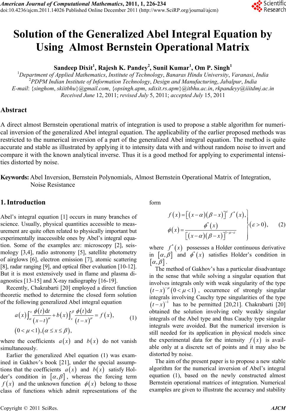