American Journal of Computational Mathematics, 2011, 1, 209-218
doi:10.4236/ajcm.2011.14024 Published Online December 2011 (http://www.SciRP.org/journal/ajcm)
Approximate Solution of the Singular-Perturbation
Problem on Chebyshev-Gauss Grid
Mustafa Gülsu, Yalçın Öztürk
Department of Mathematics, Faculty of Science, Mugla University, Mugla, Turkey
Received April 27, 2011; revised May 24, 2011; accepted June 5, 2011
Abstract
Matrix methods, now-a-days, are playing an important role in solving the real life problems governed by
ODEs and/or by PDEs. Many differential models of sciences and engineers for which the existing method-
ologies do not give reliable results, these methods are solving them competitively. In this work, a matrix
methods is presented for approximate solution of the second-order singularly-perturbed delay differential
equations. The main characteristic of this technique is that it reduces these problems to those of solving a
system of algebraic equations, thus greatly simplifying the problem. The error analysis and convergence for
the proposed method is introduced. Finally some experiments and their numerical solutions are given.
Keywords: Singular Perturbation Problems, Two-Point Boundary Value Problems, The Shifted Chebyshev
Polynomials, Approximation Method, Matrix Method
1. Introduction
The boundary-value problems for singularly perturbed
delay-differential equations arise in various practical
problems in biomechanics and physics such as in varia-
tional problem in control theory. These problems mainly
depend on a small positive parameter and a delay pa-
rameter in such a way that the solution varies rapidly in
some parts of the domain and varies slowly in some
other parts of the domain. Moreover, this class of prob-
lems possess boundary layers, i.e. regions of rapid
change in the solution near one of the boundary points.
There is a wide class of asymptotic expansion methods
available for solving the above type problems. But there
can be difficulties in applying these asymptotic expan-
sion methods, such as finding the appropriate asymptotic
expansions in the inner and outer regions, which are not
routine exercises but require skill, insight and experi-
mentation. The numerical treatment of singularly per-
turbed problems present some major computational dif-
ficulties and in recent years a large number of special-
purpose methods have been proposed to provide accurate
numerical solutions [1-5] by Kadalbajoo. This type of
problem has been intensively studied analytically and it
is known that its solution generally has a multiscale
character; i.e. it features regions called “boundary lay-
ers” where the solution varies rapidly. And these equa-
tions as well as numerical methods have been studied by
several authors [6-10]. The outer solution corresponds to
the reduced problem, i.e., that obtained by setting the
small perturbation parameter to zero. In recent years, the
Chebyshev method has been used to find the approxi-
mate solutions of differential, difference, integral and
integro-differential-difference equations [11,12]. The main
characteristic of this technique is that it reduces these
problems to those of solving a system of algebraic equa-
tions, thus greatly simplifying the problem.
Consider the of singularly-perturbed delay differential
equations form
()() ()()()=()yx pxyxqxyxgx





 (1)
where 0< <1
x
, with the boundary conditions 0 (0) =y

,
1
(1) =y

and

is a small positive parameter 0< 1

,

is also a small shifting parameter 0< 1

, ,
, ,
()px
()qx ()rx ()
s
x and ()
f
x are sufficiently smooth
functions. Our goal is to find an approximate solution
expressed polynomial of degree in the form
N
*
=0
()= ()
N
Nrr
r
yx aTx
 (2)
where r unknown coefficients, is the shifted
Chebyshev polynomials of the first kind and is cho-
sen any positive integer such that . To obtained a
solution (2) of the problem (1), we can use the zeroes of
a*()
r
Tx
Nm

N

M. GÜLSU ET AL. 210
the shifted Chebyshev polynomials of the first
kind defined by
*
1()
N
Tx

1
3π
12
=1cos ,=1,, 1
2
i
ni
xiN
N





 







 


(3)
2. Basic Idea
Polynomials are the only functions that a computer can
evaluate exactly, so we make approximate functions


,ab  by polynomials. The uniform norm (or
Chebyshev norm, maximum norm) is defined by

,
=max
xab ( ).
f
fx


Definition 2.1. For a given continuous function


,
f
Cab
N
, a best approximation polynomial of degree
is a polynomial

*
N
N
pf such that



*=min :
N
N
fpffp p



It is a good idea to approximate function by polyno-
mials, because the classical Weierstrass Theorem is a
fundamental result in the approximation of continuous
functions by polynomials [13-15].
Theorem 2.2. Let


,
f
Cab. Then for any >0

,
there exists a polynomial for which p.fp



Proof: See Ref. [13-16].
Theorem 2.3. For any


,
f
Cab

and the
best approximation polynomial
0N

*
N
pf exists and is
unique.
Proof: See Ref. [13-16].
Definition 2.4. Given an integer then a grid
set of points are 0iN in
1N

1N
 
=i Xx


,ab
0
()
ii
x
such
that 01 . Then pointsare
called the nodes of the grid.
<<<
N
xax xbN
Theorem 2.5. Given a function


,
f
Cab
N
and a
grid of nodes,

1N

0
()
ii
Xx

, there exists a
unique polynomial of degree , NN

X
I
f such that


=,0
Ni i

X
I
fx fxiN

X
N
I
f is called the interpolant (or the interpolating
polynomial) of
f
through the grid
X
.
Proof: See Ref. [13-16].
The interpolant

X
N
I
f can be express in the La-
grange form as
  
=0
=
N
XX
Ni
i
i
I
ffx
x
where

X
i
x
 is the i-th Lagrance cardinal polynomial
associated with the grid
X
:
0,
(),0.
Nj
X
i
jij
ij
x
x
x
iN
xx






The Lagrange cardinal polynomials are such that


,0 ,.
X
ij ij
x
ij N 


The best approximation polynomial


*
N
pf is also
an interpolant of
f
at


1N nodes the error is given
by formula:



 
*
1
X
NNN
f
If Xfpf



where


N
X
 is the Lebesgue constant relative to the
grid
X
,



,0
:max
NX
Ni xab
i
X
x

 
The Lebesgue constant contains all the information on
the effects of the choice of
X
on

.
X
N
fI f


Theorem 2.6. For any choice of the grid
X
, there
exist a constant such that
>0C
 
2ln 1
π
N
X
NC


)
Proof: See Ref. [13-16].
Definition 2.7. The nodal polynomial associated with
the grid is the unique polynomial of degree (1N

and
leading coefficient 1 whose zeroes are the 1N

nodes
of
X
:

1
0
()
N
X
N
i
i
wx xx



Theorem 2.8. If


1, N
f
Cab

, then for any grid
X
1Nof

nodes, and for any


,
x
ab, the inrpola-
tion error at
te
x
is
 

(1)
1()
1!
N
XX
NN
f
f
xI fxwx
N




 (4)
where


=() ,
x
ab   and nodal polyno-
mial associated with the grid 1()
X
N
wx

X
.
Proof: See Ref. [13-16].
2.1. The Shifted Chebyshev Polynomial of the
First Kind
Definition 2.9. The Chebyshev polynomial of the first
kind is a polynomial in ()
n
Tx
x
of degree , defined
by the relation [17]
n


( )coswhencos.
n
Tx nx


 
If the range of the variable
x
is the interval[1,1]

,
the range the corresponding variable

can be taken
. Since the range is quite often more con-
venient to use than the range, we map the inde-
pendent variable
[0, π][0,1 ]
[1,1]
x
in to the variable[0,1]
s
in [1,1]

by the transformation


M. GÜLSU ET AL. 211
2.2. Chebyshev-Gauss Grid

1
21or1
2
s
xx s
Definition 2.10. The grid 0
iiN
such that the
i

Xx


x
’s are the 1N

zeroes of the Chebyshev polynomial
of degree 1N

is called the Chebshev-Gauss (CG)
grid.
and this lead to a shifted Chebyshev polynomial of the
first kind of degree in
*()
n
Tx n
x
on given
by [17]
[0,1]

*()=()=21.
nnn
Tx TsTx Theorem 2.11. The polynomials of degree 1N

and
leading coefficient 1, the unique polynomial which has
the smallest uniform norm on is the
[1,1](n1)

-th
Chebyshev polynomial divided by .
2N
Thus we have the polynomials
** *2
01 2
()=1,()=2 1,()=88 1,TxTxx Txxx Proof: See Ref. [13-16].
It is of course possible to defined , like ,
directly by a trigonometric relation. Indeed, we obtained
*()
n
Tx ()
n
Tx 3. Fundamental Matrix Relations
*2
( )cos2whencos.
n
Txnx x  
This relation might alternatively be rewritten, with

replace by 2

, in the form
  
*2
1
( )coswhencos1cos
22
n
Tx x








Let us consider the Equation (1) and find the matrix
forms of each term of the equation. We first consider the
solution and its derivative
()
N
yx ()
()
m
N
y
x defined by
a truncated Chebyshev series. Then we can put series in
the matrix form
*(1)*(1)(2)
*(2)
()() ,()() ,()
()
NN N NN
N
yx TxAyx TxAy x
TxA

 (6)
Note that the shifted Chebyshev polynomial is
neither even nor odd and indeed all powers of x from
()
n
Tx
0
1=
x
to n
x
appear in . The leading coefficient
of
*()
n
Tx
n
x
in for to be . These poly-
nomials have the following properties:
*
n
T()x>0n21 2nwhere
*** *
01
()= ()()()
NN
TxTx TxTx





1) has exactly
*
1()
n
Tx
1n

real zeroes on the in-
terval . The m-th zero
[0,1] ,nm
x
of is located
at
*
1() n
Tx

*(1)*(1) *(1)*(1)
() 01
()= ()()()
NN
Tx TxTxTx





*(2)*(2) *(2)*(2)
() 01
()= ()()()
NN
Tx TxTxTx





,
3π
12
1cos
2
nm
nm
xn













 



01
=T
N
Aaa a



By using (5), we obtained the corresponding matrix
relation as follows:

1
**
()()andso ()()
TT
NN
Xx DT xTxXxD
T

 (7)
2) It is well known that the relation between the pow-
ers n
x
and the shifted Chebyshev polynomials
is
*()
n
Tx
where
()=1 N
X
xxx





*
21=0
2
1
=
2
n
n
nk
n
k
n().
x
Tx
k




 (5) and
0
21
43 3
221 2121
0
200 0
0
22
202 0
12
=44 4
22 20
23 4
22 2
22 22
12
NN NN
D
NN N
NN N

 
 
2
2
N
N











 


 


 


 


 


 






 


 



 





 


M. GÜLSU ET AL. 212
Moreover it is clearly seen that the relation between
the matrix ()
X
x and its derivative () ()
k
X
x,
1 (2)(1)2
()= (),()= ()
X
xXxBXxXxB (8)
where
010 0
002 0
=.
000
000 0
B
N










 


The derivative of the matrix defined in (7), by
*()
N
Tx
using the relation (8), can expressed as


1
*( )( )1
()()() ,0,1,2
kkT kT
N
TxXxDXxBD k

 (9)
where ,
*(0) *
()= ()
NN
TxTx (0) ()= ()
X
xXx, . By
substituting (9) into (6), we obtain
0=BB

1
()
()=(),=0,1,2
kkT
N
yxXxBD Ak
 (10)
where (0) ()= ()
NN
y
xyx.
Moreover, we know that;


=
X
xXxB

  (11)
where
01 2
01
02
0
012
() ()()()
012
12
0()() ()
01 1
=2
00()()
02
000 ()
0
N
N
N
N
N
N
N
BN
N
N


 





 
 
  
 


 

 
 


 

 


 


 















1
Using relation (8) and (11), we can write
(1) 1
()=()
X
xXxBB

  (12)
In a similarly way as (10) , we obtain
 

1
(1) *(1).
T
N
yxT xAXxBBD A



  (13)
Matrix Representation of the Conditions
Using the relation (10), the matrix form of the conditions
given by (2) can be written as
 


 


1
00
1
11
00
11
T
T
yXDA
yXDA





 
 
(14)
where
 

0=1 00X




1=1 11.X
4. Method of Solution
We are ready to construct the fundamental matrix equa-
tion corresponding to Equation (1). For this propose,
firstly substituting the matrix relation (10) and (13) into
(1) we obtained


 


 



11
2
1
TT
T
XxB DpxXxBB D
qxX xDAgx







(15)
For computing the Chebyshev coefficient matrix A
numerically, the zeroes of the shifted Chebyshev poly-
nomials of the first kind defined by (3) are putting above
relation (15) and organized. We obtained,


 


 



111
2TTT
iii iii
X
xBDpxXxBBDqxXxDA gx



 
So, the fundamental matrix equation is gained



111
2TTT
EXBDPXBBDQX DAG


 
here
(16)
w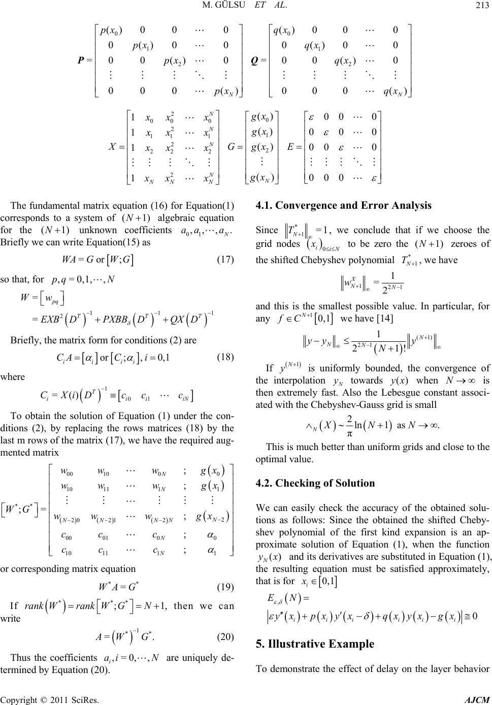

M. GÜLSU ET AL.213








0
00
11
22
()000() 000
0()000()0 0
=00()0=00 ()0
000()0 00()
NN
px qx
px qx
px qx
px qx











 

PQ
2
0
00 0
2
1
11 1
2
2
222
2
() 00 0
1
() 00
1
() 00 0
1
() 000
1
N
N
N
N
N
NN N
gx
xx x
gx
xx x
XGgxE
xx x
gx
xx x







































 



 


The fundamental matrix equation (16) for Equation(1)
corresponds to a system of (1)N algebraic equation
for the (1)N unknown ients 01 ,, ,.coeffic
N
aa a
Briefly weite Equation(15) as

can wr

=or ;WAGWG (17)
so that, for
1
T

Briefly, the matrix form for conditions (2) are
,=0,1,,pq N

11
2
=
pq
TT
EXB DPXBBDQXD





=Ww 




or; ,0,1
ii ii
CACi   (18)
where



1
01
=()T
iii
CXiDc cc

iN
To obtain the solution of Equation (1) underthe con-
di tions (2), by replacing the rows matrices (18) by the
last m rows of the matrix (17), we have the required aug-
mented matrix



 

00 1000
10 1111
**
2
20 212
00 0100
10 1111
;
;
;= ;
;
;
N
N
N
NN NN
N
N
w gx
wwwgx
WG www gx
cc c
cc c







 








 



ww





or corresponding matrix equation
(19)
If
**
=WA G

***
;
1
rank WrankWGN




w
, then we can
rite

1
**
=.
A
WG
 (20)
Thus the coefficients are uniquely de-
termined by Equation (2
4.1. Convergence and Error Analysis
,=0, ,
i
ai N
0).
Since *
1=1 N
T, we conc

grid nodes
lude that if we choose the


0
iiN
x

 to be zero the (1N)
zeroes of
hebysthe shifted Chev polynomial 1N T, we have
*
121
1
=
X
NN
w
2

and this is the smallest possible value. particular, In for
any


10,1 N
fC

 we have [14]

(1)
21
21 !
N
NN
yy y
N



 
1
If

1N
y

the interpolation
is uniformly bounded, the convence of erg
towards ()
y
x
besgue
N
y when is
then eely fastAlso the Le co
atith th

nstant associ-
N
xtrem.
ed we Chebyshev-Gauss grid is small
 
2ln1as.
π
NXNN

 
This is much better than uniform grids and close to the
optimal value.
4.
We can easily check the accuracy of the obtained solu-
tained the shifted Cheby-
shev polynomial of the first kind expansion is an ap-
2. Checking of Solution
tions as follows: Since the ob
proximate solution of Equation (1), when the function
()
N
yx and its derivatives are substituted in Equation (1),
the resulting equation must be satisfied approximately,
that is for


0,1
i
x


 
,
i
EN
yx x



 0
ii iii
pxyqxyx gx 

 
5. Illustrative Example
To demonstrate the effect of delay on the layer behavior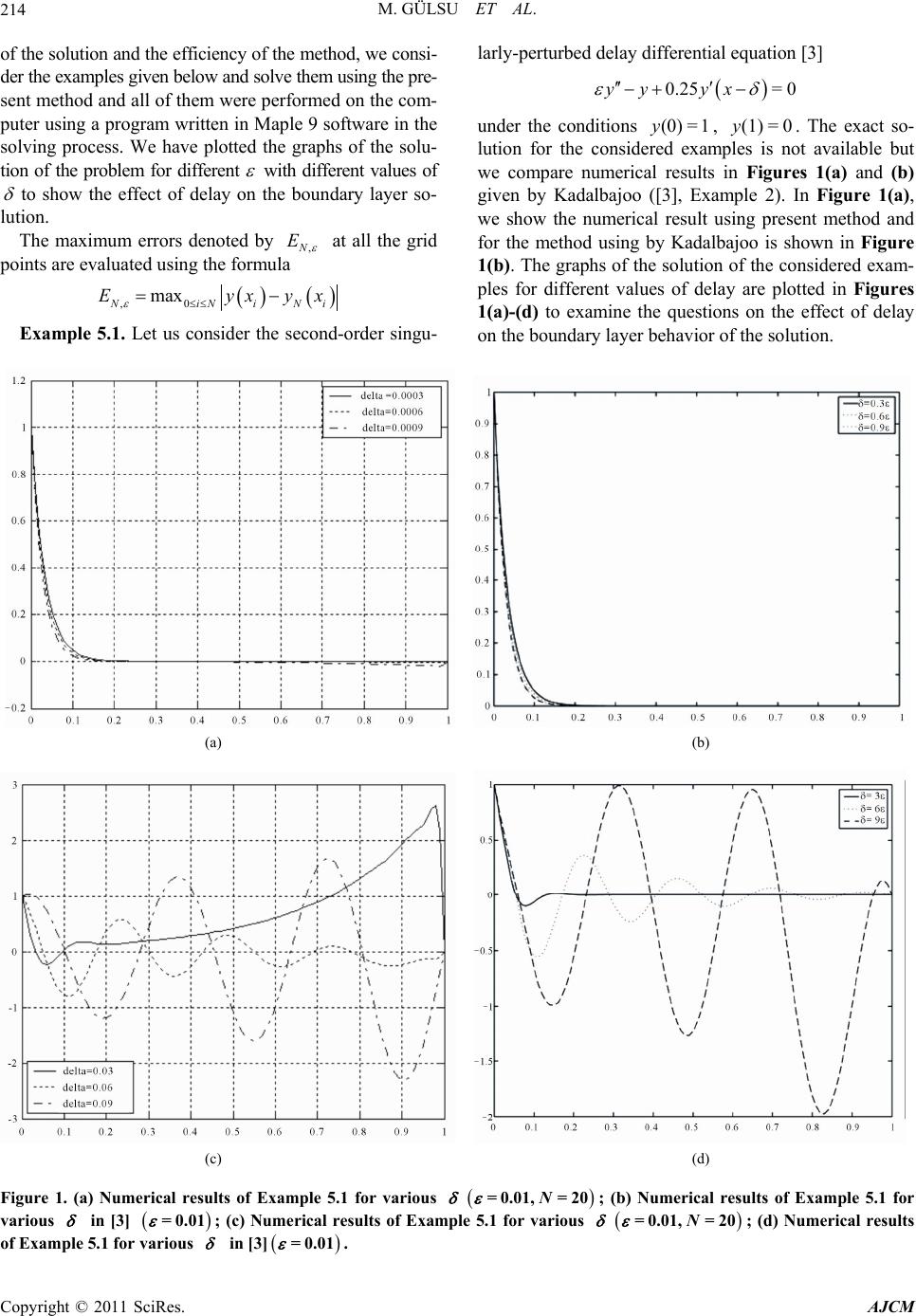

M. GÜLSU ET AL. 214
of the method, we consi-
der the examples given below and solve them using the pre-
of the solution and the efficiency
sent method and all of them were performed on the com-
puter using a program written in Maple 9 software in the
solving process. We have plotted the graphs of the solu-
tion of the problem for different

with different values of

to show the effect of delay on the boundary layer so-
lution.
The maximum errors denotedy ,N
E
b

at all the grid
ints are evaluated using the formula po


,0
max
N
iN ii
Eyx
 

Example 5.1. Let us consider the sec
N
yx
ond-order singu-
la
under the conditions
lution for the considered examples is not available but
l resultFigur
rly-perturbed delay differential equation [3]

0.25=0yy yx 
 

(0)= 1y, (1)= 0y. The exact so-
we compare numericas in es 1(a) and (b)
given by Kadalbajoo ([3], Example 2). In Figure 1(a),
we show the numerical result using present method and
for the method using by Kadalbajoo is shown in Figure
1(b). The graphs of the solution of the considered exam-
ples for different values of delay are plotted in Figures
1(a)-(d) to examine the questions on the effect of delay
on the boundary layer behavior of the solution.
(a) (b)
(c) (d)
Figure 1. (a) Numerical results of Example 5.1 for various



= 0.01,= 20  N; (b) Numerical results of Example 5.1 for
various

in [3]


=0.01  ; (c) Numerical results of Example 5.1 for various



= 0.01,= 20  N; (d) Numerical results
of Example 5.1 for various

in [3]


=0.01  .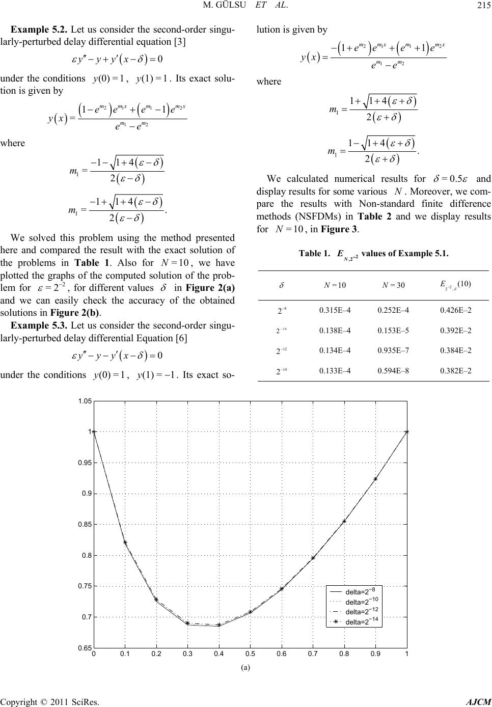

M. GÜLSU ET AL.215
nse seconder singu-
under the conditions . Its exact solu-
Example 5.2. Let us coider th-ord
larly-perturbed delay differential equation [3]

0yyyx 
 
 
(0)= 1y, (1)= 1y
tion is given by


21 12
12
11
=
mmx mmx
mm
ee ee
yx ee


where


1
114
=2 m



 



1
114
=.
2
m



 

We solved this problem using the method presented
here and compared the result with the exact solution of
the problems in Table 1. Also for =10N, we have
plotted the graphs of the computed solutiof the prob-
lem for 2 =2 
, for different values
n o

in Figure 2(a)
and we casily check the accuracy of the obtained
solutions in Figure 2(b) .
Example 5.3. Let us consider the second-order singu-
la
n ea
rly-perturbed delay differential Equation [6]

0yyyx 
 

under the conditions . Its exact so-
lution is given by
(0)= 1y, (1) =1y



21 12
12
11
mmx mmx
mm
ee ee
yx ee
 

where


1
114
2
m



 



1
114 .
2
m



 

We calculated numerical results for =0.5

 and
di
Table 1.
splay results for some various N. Moreover, we com-
pare the results with Non-standard finite difference
methods (NSFDMs) in Table 2 and we display results
for =10N, in Figure 3.
2
,2

N
Evalues of Example 5.1.

=10N =30N 2
2,
(10)E


8
2

0.315E–4 0.252E–4 0.426E–2
10
2 0.138E–4 0.153E–5 0.392E–2
12
2 0.134E–4 0.935E–7 0.384E–2
14
2 0.133E–4 0.594E–8 0.382E–2
00.10.20.3 0.4 0.50.60.7 0.80.91
0.65
0.7
0.75
0.8
0.85
0.9
0.95
1
1.05
delta=2
−8
delta=2
−10
delta=2
−12
delta=2
−14
(a)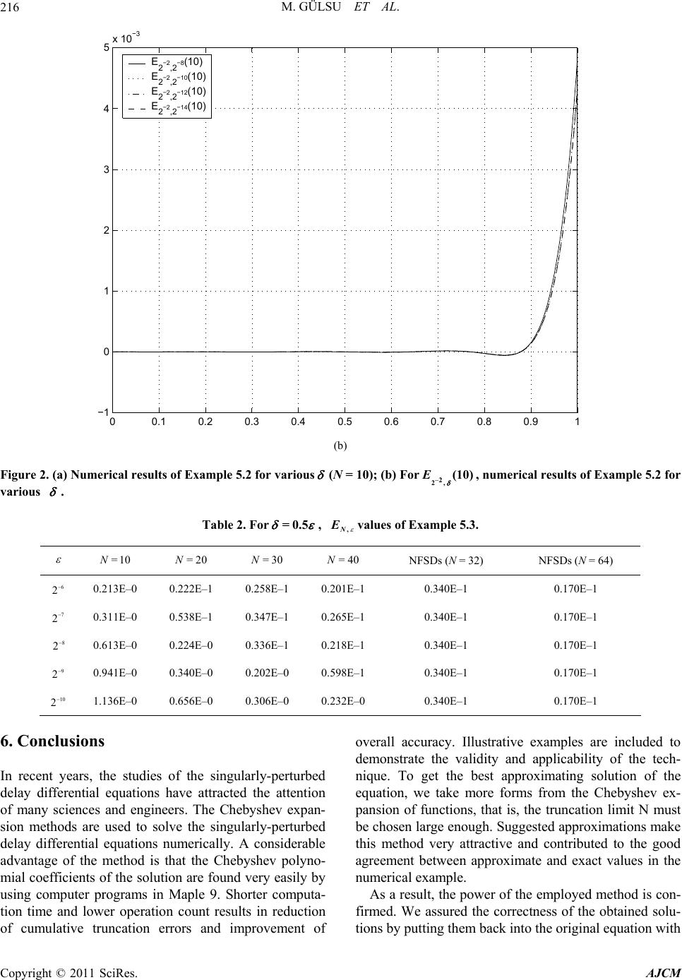

M. GÜLSU ET AL. 216
00.1 0.2 0.3 0.4 0.5 0.60.70.8 0.9
1
−
1
0
1
2
3
4
5x 10
−3
E
2
−2
,2
−8(10)
E
2
−2
,2
−10(10)
E
2
−2
,2
−12(10)
E
2
−2
,2
−14(10)
(b)
Figure 2. (a) Numerical results of Example 5.2 for various(N = 10); (b) For, numerical results of Example 5.2 for

2
2,(10)E

various

.
Table 2. For=0.5

 ,

,N
Evalues of Example 5.3.

=10N =2N0 =3N NFSDs (N = 32)
0 =40NNFSDs (N = 64)
6
2 0.213E–0 0.222E–1 0.258E–1 0.201E–1 0.340E–1 0.170E–1
7
2 0.311E–0 0.538E–1 0.347E–1 0.265E–1 0.340E–1 0.170E–1
8
2 0.613E–0 0.224E–0 0.336E–1 0.218E–1 0.340E–1 0.170E–1
9
2 0.941E–0 0.340E–0 0.202E–0 0.598E–1 0.340E–1 0.170E–1
10
2 1.136E–0 0.656E–0 0.306E–0 0.232E–0 0.340E–1 0.170E–1
studies of the singularly-perturbed
overall accuracy. Illustrative examples are included to
tions by putting them back into the original equation with
6. Conclusions
In recent years, the
delay differential equations have attracted the attention
of many sciences and engineers. The Chebyshev expan-
sion methods are used to solve the singularly-perturbed
delay differential equations numerically. A considerable
advantage of the method is that the Chebyshev polyno-
mial coefficients of the solution are found very easily by
using computer programs in Maple 9. Shorter computa-
tion time and lower operation count results in reduction
of cumulative truncation errors and improvement of
demonstrate the validity and applicability of the tech-
nique. To get the best approximating solution of the
equation, we take more forms from the Chebyshev ex-
pansion of functions, that is, the truncation limit N must
be chosen large enough. Suggested approximations make
this method very attractive and contributed to the good
agreement between approximate and exact values in the
numerical example.
As a result, the power of the employed method is con-
firmed. We assured the correctness of the obtained solu-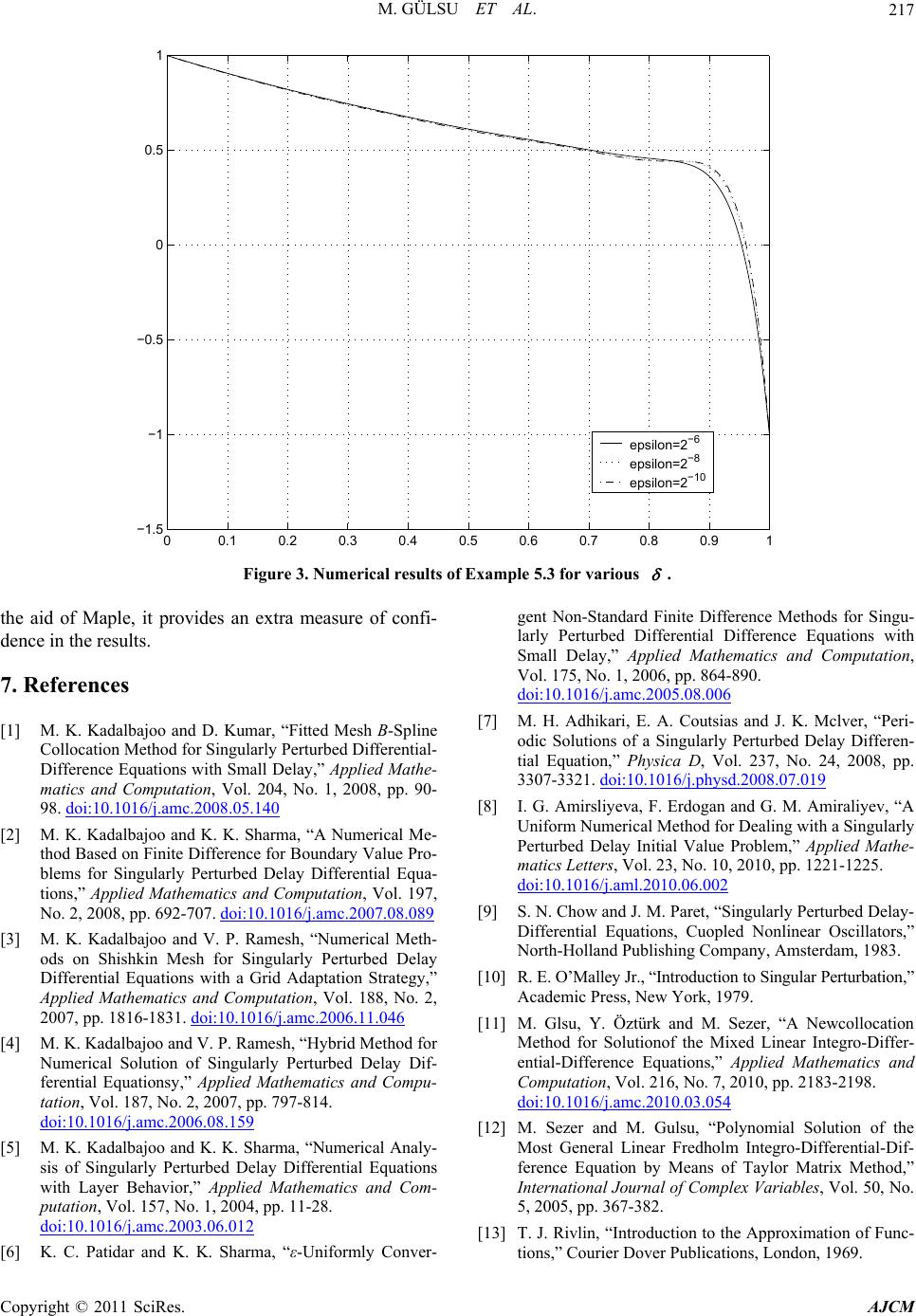

M. GÜLSU ET AL.217
00.1 0.2 0.3 0.40.5 0.6 0.7 0.8 0.9
1
−
1.5
−1
−
0.5
0
0.5
1
epsilon=2
−6
epsilon=2
−8
epsilon=2
−10
Figure 3. Numerical results of Example 5.3 for various

.
the aid of Maple, it provides an extra measure of confi-
dence in the results.
Kumar, “Fitted Mesh B-Spline
ethod for Singularly Perturbed Differential-
ations with Small Delay,” Applied Mathe-
7. References
[1] M. K. Kadalbajoo and D.
Collocation M
Difference Equ
matics and Computation, Vol. 204, No. 1, 2008, pp. 90-
98. doi:10.1016/j.amc.2008.05.140
[2] M. K. Kadalbajoo and K. K. Sharma, “A Numerical Me-
thod Based on Finite Difference for Boundary Value Pro-
blems for Singularly Perturbed Delay Differential Equa-
tions,” Applied Mathematics and Computation, Vol. 197,
No. 2, 2008, pp. 692-707. doi:10.1016/j.amc.2007.08.089
[3] M. K. Kadalbajoo and V. P. Ramesh, “Numerical Meth-
ods on Shishkin Mesh for Singularly Perturbed Delay
Differential Equations with a Grid Adaptation Strategy,”
Applied Mathematics and Computation, Vol. 188, No. 2,
2007, pp. 1816-1831. doi:10.1016/j.amc.2006.11.046
[4] M. K. Kadalbajoo and V. P. Ramesh, “Hybrid Method for
Numerical Solution of Singularly Perturbed Delay Dif-
ferential Equationsy,” Applied Mathematics and Compu-
tation, Vol. 187, No. 2, 2007, pp. 797-814.
doi:10.1016/j.amc.2006.08.159
[5] M. K. Kadalbajoo and K. K. Sharma, “Numerical Analy-
sis of Singularly Perturbed Delay Differential Equations
with Layer Behavior,” Applied Mathematic
putation, Vol. 157, No. 1, 2004,
s and Com-
pp. 11-28.
doi:10.1016/j.amc.2003.06.012
[6] K. C. Patidar and K. K. Sharma, “ε-Uniformly Conver-
Vol. 175, No. 1, 2006, pp. 864-890.
gent Non-Standard Finite Difference Methods for Singu-
ffntial Difference Equations with
li Mathematics and Computation,
larly Perturbed Diere
Small Delay,” App ed
doi:10.1016/j.amc.2005.08.006
[7] M. H. Adhikari, E. A. Coutsias and J. K. M
odic Solutions of a Singularly P
clver, “Peri-
erturbed Delay Differen-
tial Equation,” Physica D, Vol. 237, No. 24, 2008, pp.
3307-3321. doi:10.1016/j.physd.2008.07.019
[8] I. G. Amirsliyeva, F. Erdogan and G. M. Amiraliyev, “A
Uniform Numerical Method for Dealing with a Singularly
Perturbed Delay Initial Value Problem,” Applied Mathe-
matics Letters, Vol. 23, No. 10, 2010, pp. 1221-1225.
doi:10.1016/j.aml.2010.06.002
[9] S. N. Chow and J. M. Paret, “Singularly Perturbed Delay-
Differential Equations, Cuopled Nonlinear Oscillators,”
North-Holland Publishing Company, Amsterdam, 1983.
[10] R. E. O’Malley Jr., “Introduction to Singular Perturbation,”
Academic Press, New York, 1979.
[11] M. Glsu, Y. Öztürk and M. Sezer, “A Newcollocatio
Method for Solutionof the Mix
n
ed Linear Integro-Differ-
ential-Difference Equations,” Applied Mathematics and
Computation, Vol. 216, No. 7, 2010, pp. 2183-2198.
doi:10.1016/j.amc.2010.03.054
[12] M. Sezer and M. Gulsu, “Polynomial Solution of the
Most General Linear Fredholm Integro-Differential-Dif-
ference Equation by Means of Taylor Matrix Method,”
International Journal of Complex Variables, Vol. 50, No.
5, 2005, pp. 367-382.
[13] T. J. Rivlin, “Introduction to the Approximation of Func-
tions,” Courier Dover Publications, London, 1969.

M. GÜLSU ET AL. 218
proximation,” Dover Pub- and Fourier Spectral Methods,”
yno-
mials,” Chapman and Hall/CRC, New York, 2003.
[14] P. J. Davis, “Interpolation and Ap
lications, New York, 1963.
[15] K. Atkinson and W. Han, “Theoretical Numerical Analy-
sis,” 3rd Edition, Springer, 2009.
[16] J. P. Body, “Chebyshev
University of Michigan, New York, 2000.
7] J. C. Mason and D. C. Handscomb, “Chebyshev Pol[1