iBusiness, 2011, 3, 383-389
doi:10.4236/ib.2011.34051 Published Online December 2011 (http://www.SciRP.org/journal/ib)
383
Ordinal Logistic Regression for the Estimate of the
Response Functions in the Conjoint Analysis
Amedeo De Luca
Dipartimento di Scienze Statistiche, Università Cattolica del Sacro Cuore di Milano, Milan, Italy.
Received June 28th, 2011; revised August 29th, 2011; accepted September 28th, 2011.
ABSTRACT
In the Conjoint Analysis (COA) model proposed here—a new approach to estimate more than one response function—
an extension of the traditional COA, the polytomous response variable (i.e. evaluation of th e overall desirability of al-
ternative product profiles) is described by a sequence of binary variables. To link the categories of overall evaluation to
the factor levels, we adopt—at the aggregate level—an ordinal logistic regression, based on a main effects experimen-
tal design. The model provides several overall desirability functions (aggregated part-worths sets), as many as the
overall ordered categories are, unlike the traditiona l metric and non metric COA, which gives only one response func-
tion. We provide an application of the model and an interpretation of the main effects.
Keywords: Aggregate Level Analysis, Conjoint Analysis, Ordinal Logistic Regression, Respon se Fun c t i on
1. Introduction
Since the 1970s, Conjoint Analysis (COA) has received
considerable attention as a major set of techniques for
measuring buyers’ trade-offs among multiattributed pro-
ducts and services [1].
Since that time many new developments in COA have
been reported.
The purpose of this article is to give a new contri-
bution to the problem of the conjoint measurement in
order to quantify judgmental data.
The model proposed here is an extension of the tradi-
tional COA approach.
While in the traditional full-profile COA [1] the re-
spondent expresses preferences by rating or ranking distinct
product profiles, in our model we assume that the re-
spondent evaluative judgement Yk on the overall desir-
ability consists in a choice of one of the k (k = 1, 2, ···, K)
desirability categories for each of S hypothetical product
profiles, chosen from a sample of respondents.
The proposed approach also differs from the
“Choice-Based Conjoint” analysis (CBC) model in
which the respondent expresses preferences by choos-
ing concepts from sets of concepts (discrete choice
modelling).
In the proposed approach the ordinal response variable
is described by an ordered logit model, that directly in-
corporates the order of the categories of the Yk.
To link the categories of overall evaluation to the fac-
tor levels, we adopt a cumulative logit model [2] at the
aggregate level (pooled model) [3].
The main novelty value in our approach—which is a
further development—is that one set of aggregated part-
worths is estimated in connection with each category Yk,
as many as the overall ordered categories are (K), unlike
the traditional metric and non metric COA and CBC
analysis, which give only one set of aggregated part-
worths (response function).
Thus with our approach it is possible to make a
cross-check of the effects of the attribute levels on the
different k categories of Yk.
Moreover, the proposed model provides the following
advantages: the use of the probability Pks as an average
response, which does not require preliminary scale ad-
justments to render the preference scale “metric” (in the
non metric COA) and a cross-check of the effects of the
attribute levels on the different categories of the overall.
This allows us to verify the basic coherence of the re-
sults of the model, unlike the classical approach adopted
in literature.
This paper is structured as follows: after the presen-
tation of the proposed model and the estimation method
of response functions (the cumulative logit model), a
concrete application of the approach follows; then the
meaning of the proposed interpretative model and some
empirical results are described, to conclude with a

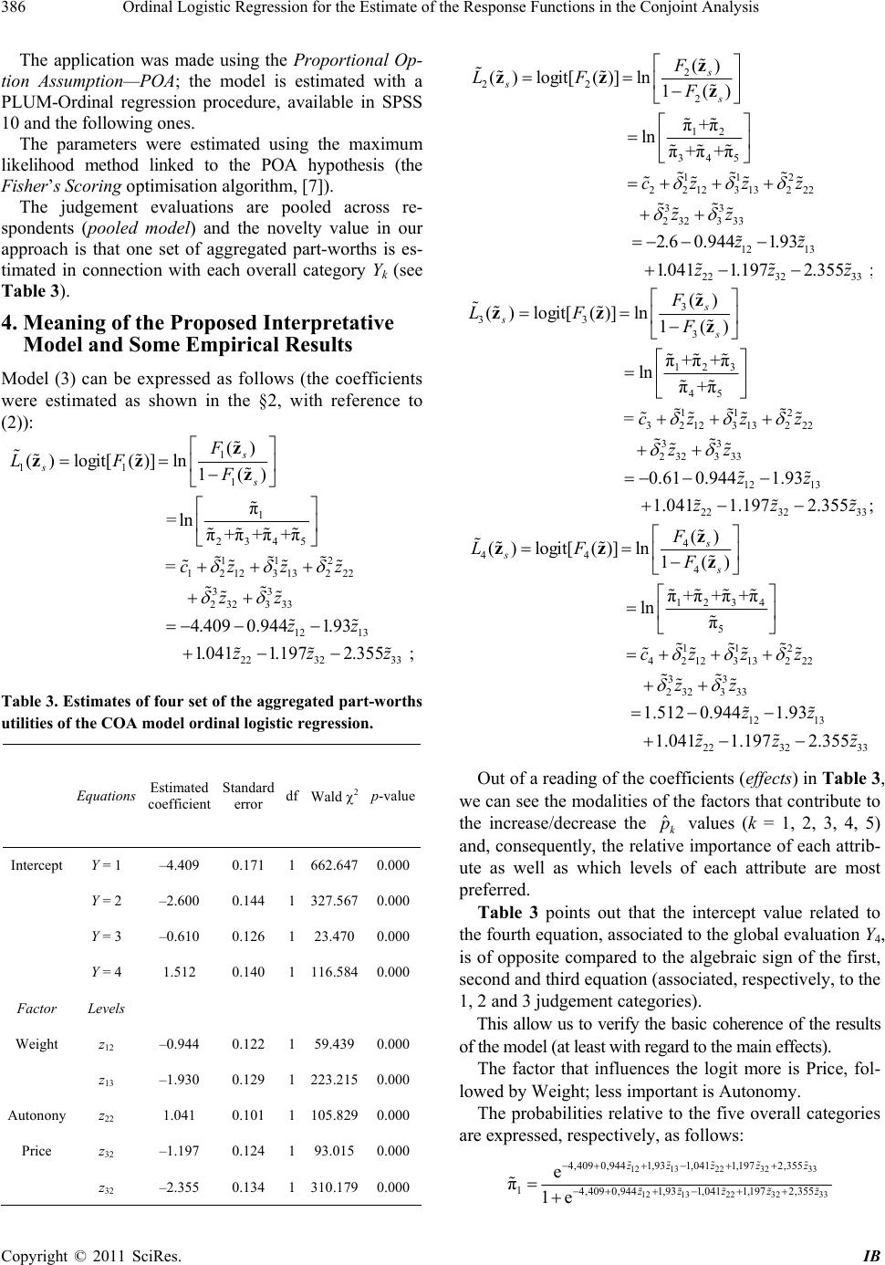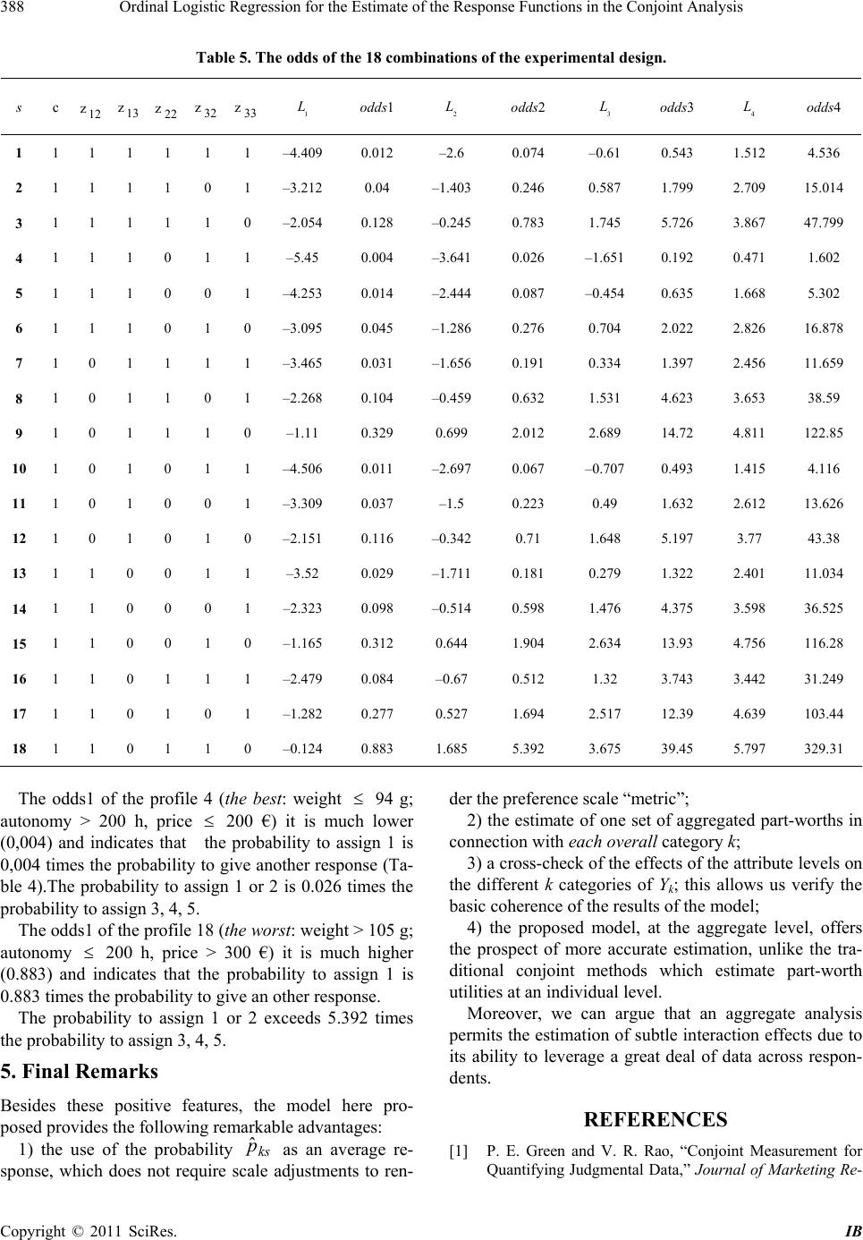
Ordinal Logistic Regression for the Estimate of the Response Functions in the Conjoint Analysis
384
statement of the benefits offered by the proposed
model—compared to the approaches known in litera-
ture—as far as the methodology of the COA is con-
cerned.
2. Estimation of Response Functions in the
Conjoint Analysis: The Cumulative Logit
Model
The cumulative logit model proposed here (that directly
incorporates the order of the categories of the overall
desirability of alternative concepts of the product) con-
cerns the full-profile coa. It is based on overall desirabil-
ity categories chosen by a sample of respondents, for
each of S hypothetical product profiles.
The number of profiles S, resulting from the total
number of possible combinations of levels of the M at-
tributes or factors (X) of a product, constitute a full-fac-
torial experimental design.
The focus of our paper is to estimate the relationship
between dependent and independent variables.
It is assumed that the global or overall evaluation
(polytomous dependent ordinal variable Y) of a product
consists in the choice of one of the ordered categories k =
1, 2, ··· K (in our application K = 5) on scale 1 - 5 (1 =
“less desirable”, 5 = “most desirable”).
In terms of probabilities, the effects of the factors ex-
press the variations of the probabilities Pks—if k is the
overall category—associated with the vector
s
z
 corre-
sponding to the combination s (s = 1, 2, ··· , S) of levels
of the M factor, as follows:



'
'
exp
(1|)
1+ exp
ks
ks
ks
ks
PY
F



 

z
zz
z




(1)
where
k

is the intercept term in regression;
'

 is the unknown vector of regression coefficients of
the factors;
s
z
is the vector of the indicator explanatory variables
relative to the combination or profile s;
Fk(
s
z) =


|

s
PY kz
is the cumulative probability for
response category k, when the explanatory variables take
the value
s
z
.
When we have a simple random sample of J respon-
dents, for the formula (1), the sample likelihood turns out
to be:

 
1
''
1
()1
j
j
Jyy
j
j
LF F  





zz

j


(2)
where
j
z
, j = 1, 2, ···, J, summarizes the underlying condi-
tions related to the generic j-th respondent of the sam-
ple;
yj = 1 if the value of the dichotomized overall evalua-
tion is Yj = 1. This is obtained by placing in the first
class all the evaluations with desirability judgement of
class greater than or equal to a given category k and
placing in the other the remaining ones (ordinal logistic
regression).
It is shown that, under suitable conditions, regarding
the behaviour of the arrays
j
z
 as long as J increases, if
the system of likelihood ln L0
k


, k = 1, 2, … K,
has a solution, this is of absolute maximum, and defines
a consistent estimator

 of the parametric vector

,
asymptotically normally distributed. See, for example,
[4].
To estimate said probabilities s
we use
an aggregate level model across the J homogeneous re-
search respondents [5], whose evaluations, on each
product profile, are considered J repeated observations.

1|
k
PYz


At this point it is necessary to estimate the relationship
between Yk (k = 1, 2, ···, K) dependent variable (overall
judgment category) and m = 1, 2, ..., M (in our applica-
tion M = 3) qualitative independent variables (product
attributes or factors X), with levels l = 1, 2, ···, lm (in our
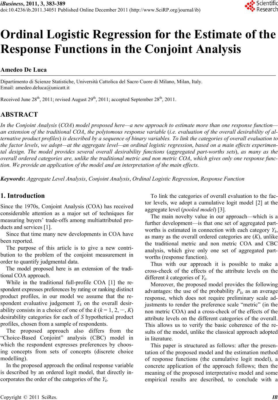
application: l1 = 3; l2 = 2, l3 = 3).
The K overall categories (Yk) are codified as K indica-
tor variables. Also the independent variables are codified
as Z indicator variables (for each variable we have de-
fined a set of 0-1 indicator variables ()m
l
Z
, l = 1, 2, ···, lm,
so that—for one m factor –()m
l
Z
= 1 if category lth is
observed, while in the all other cases ()m
l
Z
= 0).
To obtain univocal estimates of the parameters, the
column concerning the first variable of each set has been
dropped. Therefore the kth cumulative response probability
is:




 
12
(|)
π π π,
1, 2, ,,
kssk s
ss k
PYk F
kK



zz
zz z

  

s
(2)
where 
k(
s
z) is the probability of the response k associ-
ated with the reduced vector

s
z
= [1, 12 ,13 ,22 ,
32 ,33 ]'of the explicative variables that indicate the
assessment values.
zzz
z z
The cumulative probabilities reflect the ordering, with:
(1|)( 2|)(|
kss ksskss
PYPYP K)

 zz

z

where


|1
ks s
PY K

z
.
The model for cumulative probabilities does not use
the final cumulative probability

|

K
s
PYKz
s
, since it
is necessarily equal to 1.
In the configured model, owing to the interrelationship
between the K dependent variables, the Kth equation can
be drawn from the remaining q = K – 1 equations.

Ordinal Logistic Regression for the Estimate of the Response Functions in the Conjoint Analysis385
The cumulative logits of the first (K – 1) cumulative
probabilities are:
 

12
12
'
()logit ln1
() ()()
= ln() ()()
ks
ksk sks
ss ks
ksk sKs
k
F
LF F

 



 










z
zz z
zz z
zz z
z



 

  


(3)
with k = 1, 2, ···, K – 1;
where
s
z
is the vector of the reduced matrix (in which it
has been dropped out one of the indicator variables for
each level of the M factors X);
Z

k

is the constant term associated to the reference
category (the k

are called cutpoint parameters. They
are not decreasing in k, since the cumulative logit is an
increasing function of , which is itself increasing
in k for fixed

ks
Fz

s
z
);
'

 is the vector of the unknown coefficients.
In Equation (3) '

does not have a k subscript (Pro-
portional Odd Assumption—POA; see [6]) , so the model
assumes the same effects as for all K – 1 on all cu-
mulative logit results, in a parsimonious model for ordi-
nal data.
Z

When this model fits well it requires a single parameter
rather than K – 1 parameters to describe the effect of .
z

3. Application of the Cumulative Logit
Model
The model was applied to the overall desirability evalua-
tions expressed on the K = 5 categories by a sample of J
= 79 users on S = 18 new profiles of mobile phones.
The M = 3 experimental factors and levels where: X1 =
“weight” (with levels: 94 grams, 95 - 105 grams, >105
grams); X2 = “autonomy” (200 h, >200 h); X3 = “price”
(<200 €, 200 - 300 €, >300 €).


The K overall categories (Yk) are codified as K indica-
tor variables (Table 1); also the independent variables
are codified as indicator variables (Z) (Table 2).
Table 1. Disjunctive binary coding of overall evaluations (Yk)
categories.
Indicator
variables
Overall
evaluation (Yk)
Y1 Y2 Y3 Y4 Y
5
k = 1 1 0 0 0 0
k = 2 0 1 0 0 0
k = 3 0 0 1 0 0
k = 4 0 0 0 1 0
k = 5 0 0 0 0 1
Table 2. Disjunctive binary coding of factors: “weight”,
“autonomy”, “price”.
Predictor variables and levels (l) Indicator variables
Weight (1)
1
Z
(1)
2
Z
(1)
3
Z

94 grams 1 0 0
95 - 105 grams 0 1 0
>105 grams 0 0 1
Predictor variables and levels (l) Indicator variables
Autonomy (2)
1
Z
(2)
2
Z

200 h 1 0
>200 h 0 1
Predictor variables and levels (l) Indicator variables
Price (3)
1
Z
(3)
2
Z
(3)
3
Z
<200 € 1 0 0
200 - 300 € 0 1 0
>300 € 0 0 1
The reduced matrix of the indicator variables of the
experimental design is as follows (see § 2):
Z

1| 0 0|0 |00
1| 0 0|0 |10
1| 0 0|0 |01
1|00|1|00
1|00|1|10
1|00|1|01
1|1 0|0| 0 0
1|1 0|0|1 0
1|1 0| 0| 0 1
1|10|1|00
1|10|1|10
1|10|1|01
1| 0 1| 0| 0 0
1| 0 1| 0| 1 0
1| 0 1| 0| 0 1
1| 0 1|1| 0 0
1|0 1|1|10
1| 0 1|1| 0 1



































Z

























Ordinal Logistic Regression for the Estimate of the Response Functions in the Conjoint Analysis
386
The application was made using the Proportional Op-
tion Assumption—POA; the model is estimated with a
PLUM-Ordinal regression procedure, available in SPSS
10 and the following ones.
The parameters were estimated using the maximum
likelihood method linked to the POA hypothesis (the
Fisher’s Scori ng optimisation algorithm, [7]).
The judgement evaluations are pooled across re-
spondents (pooled model) and the novelty value in our
approach is that one set of aggregated part-worths is es-
timated in connection with each overall category Yk (see
Table 3).
4. Meaning of the Proposed Interpretative
Model and Some Empirical Results
Model (3) can be expressed as follows (the coefficients
were estimated as shown in the §2, with reference to
(2)):
1
11
1
1
2345
112
12 12313222
()
()logit[()] ln1()
π
=lnπ+π+π+π
=
s
ss
F
LF F
cz zz 









z
zz z






 
33
232 333
12 13
22 3233
4.4090.9441.93
1.0411.1972.355 ;
zz
zz
zzz
 
 




 
Table 3. Estimates of four set of the aggregated part-worths
utilities of the COA model ordinal logistic regression.
Equations
Estimated
coefficient
Standard
error df Wald 2p-value
Intercept Y = 1 –4.409 0.171 1 662.6470.000
Y = 2 –2.600 0.144 1 327.5670.000
Y = 3 –0.610 0.126 1 23.4700.000
Y = 4 1.512 0.140 1 116.5840.000
Factor Levels
Weight z12 –0.944 0.122 1 59.4390.000
z13 –1.930 0.129 1 223.2150.000
Autonony z22 1.041 0.101 1 105.8290.000
Price z32 –1.197 0.124 1 93.0150.000
z32 –2.355 0.134 1 310.1790.000
2
22
2
12
345
112
22 123 13222
()
()logit[()] ln1()
π+π
lnπ+π+π
s
ss
F
LF F
cz zz 








  
z
zz z







33
232 333
12 13
22 3233
2.60.9441.93
1.0411.1972.355
;
zz
zz
zz
 
 




 z 
3
33
3
123
45
112
3 212 313 222
()
() logit[ ()] ln1()
π+π+π
lnπ+π
=
s
ss
F
LF F
cz zz 









z
zz z



 


 
33
232333
12 13
22 3233
0.610.9441.93
1.0411.1972.355;
zz
zz
zz
 
 




z 
4
44
4
1234
5
112
42 12313222
()
()logit[()] ln1()
π+π+π+π
lnπ
s
ss
F
LF F
cz zz 








 
z
zz z



 



33
232 333
12 13
22 3233
1.5120.9441.93
1.0411.1972.355
zz
zz
zz
 
 




z 
Out of a reading of the coefficients (effects) in Tabl e 3 ,
we can see the modalities of the factors that contribute to
the increase/decrease the values (k = 1, 2, 3, 4, 5)
and, consequently, the relative importance of each attrib-
ute as well as which levels of each attribute are most
preferred.
ˆk p
Table 3 points out that the intercept value related to
the fourth equation, associated to the global evaluation Y4,
is of opposite compared to the algebraic sign of the first,
second and third equation (associated, respectively, to the
1, 2 and 3 judgement categories).
This allow us to verify the basic coherence of the results
of the model (at least with regard to the main effects).
The factor that influences the logit more is Price, fol-
lowed by Weight; less important is Autonomy.
The probabilities relative to the five overall categories
are expressed, respectively, as follows:
12 13223233
12 13223233
4,409 0,9441,931,0411,1972,355
14,409 0,9441,931,0411,1972,355
e
π
1e
zz zzz
z
zzzz
 
 

 
 


Ordinal Logistic Regression for the Estimate of the Response Functions in the Conjoint Analysis
387
12 13223233
12 13223233
2,6 0,9441,931,0411,1972,355
21
2,6 0,9441,931,0411,1972,355
e
ππ
1e
zz zzz
zz zzz
 
 


 
 

12 13223233
12 13223233
0,61 0,9441,931,0411,1972,355
31
0,61 0,9441,931,0411,1972,355
e
π
1e
zz zzz
zz zzz
 



 
 
2
π π

12 13223233
12 13223233
1,5120,9441,931,0411,1972,355
4123
π

1,5120,9441,931,0411,1972,355
πππ
1
zz zzz
zz zzz
e
e




 
 

4

5123
π1ππ ππ 

In order to empirically assess the predictive capacity
of the estimated model, Table 4 shows the probabilities
estimated for all the modality combinations (experiment-
tal conditions “s”) of the explanatory variables and the
corresponding values of the observed proportions.
We notice a satisfactory model fitting, as the predicted
probabilities turn out to be very near the corresponding
proportions for all the modality combinations of the ex-
perimental design.
Table 5 supplies, for each product profile “s”, the odds
value relative to the four probability functions , that
is, the values:
πk

'
1
1
2345
π
1e
π+π+π+π
odds

 




z



'
2
12
345
π+π
2e
π+π+π
odds

 




z



'
3
123
45
ππ π
3e
ππ
odds

 






z

 

'
4
123
5
4
4e odds











z

 

Table 4. Comparison of the predicted probabilities, estimated by the COA model, and the corresponding proportions for all
the modality combinations of the experimental design.
Y
1 Y 2 Y 3 Y 4 Y 5
s Probability Proportion Probability ProportionProbabilityProportionProbabilityProportion Probability Proportion
1
π()
s
z
 p1 2
π()
s
z
 p
23
π()
s
z
p
34
π()
s
z
p
45
π()
s
z
 p
5
1 0.01 0.01 0.06 0.04 0.28 0.30 0.47 0.46 0.18 0.19
2 0.04 0.04 0.16 0.20 0.45 0.41 0.29 0.30 0.06 0.05
3 0.11 0.13 0.33 0.29 0.41 0.46 0.13 0.11 0.02 0.01
4 0.00 0.00 0.02 0.01 0.14 0.14 0.45 0.44 0.38 0.41
5 0.01 0.03 0.07 0.06 0.31 0.25 0.45 0.49 0.16 0.16
6 0.04 0.06 0.17 0.15 0.45 0.49 0.28 0.24 0.06 0.05
7 0.03 0.01 0.13 0.16 0.42 0.39 0.34 0.35 0.08 0.08
8 0.09 0.08 0.29 0.28 0.43 0.49 0.15 0.14 0.03 0.01
9 0.25 0.24 0.42 0.39 0.27 0.30 0.06 0.06 0.01 0.00
10 0.01 0.00 0.05 0.06 0.27 0.24 0.47 0.51 0.20 0.19
11 0.04 0.04 0.15 0.14 0.44 0.47 0.31 0.33 0.07 0.03
12 0.10 0.13 0.31 0.33 0.42 0.35 0.14 0.19 0.02 0.00
13 0.03 0.03 0.12 0.14 0.42 0.44 0.35 0.29 0.08 0.10
14 0.09 0.04 0.29 0.33 0.44 0.46 0.16 0.14 0.03 0.04
15 0.24 0.22 0.42 0.44 0.28 0.24 0.06 0.09 0.01 0.01
16 0.08 0.08 0.26 0.29 0.45 0.44 0.18 0.13 0.03 0.06
17 0.22 0.23 0.41 0.41 0.30 0.28 0.07 0.06 0.01 0.03
18 0.47 0.49 0.37 0.29 0.13 0.18 0.02 0.03 0.00 0.01

Ordinal Logistic Regression for the Estimate of the Response Functions in the Conjoint Analysis
388
Table 5. The odds of the 18 combinations of the experimental design.
s c z
12 z
13 z
22 z32 z
33 1
L
odds1 2
L
odds2 3
L
odds3 4
L
odds4
1 1 1 1 1 1 1 –4.409 0.012 –2.6 0.074 –0.61 0.543 1.512 4.536
2 1 1 1 1 0 1 –3.212 0.04 –1.403 0.246 0.587 1.799 2.709 15.014
3 1 1 1 1 1 0 –2.054 0.128 –0.245 0.783 1.745 5.726 3.867 47.799
4 1 1 1 0 1 1 –5.45 0.004 –3.641 0.026 –1.651 0.192 0.471 1.602
5 1 1 1 0 0 1 –4.253 0.014 –2.444 0.087 –0.454 0.635 1.668 5.302
6 1 1 1 0 1 0 –3.095 0.045 –1.286 0.276 0.704 2.022 2.826 16.878
7 1 0 1 1 1 1 –3.465 0.031 –1.656 0.191 0.334 1.397 2.456 11.659
8 1 0 1 1 0 1 –2.268 0.104 –0.459 0.632 1.531 4.623 3.653 38.59
9 1 0 1 1 1 0 –1.11 0.329 0.699 2.012 2.689 14.72 4.811 122.85
10 1 0 1 0 1 1 –4.506 0.011 –2.697 0.067 –0.707 0.493 1.415 4.116
11 1 0 1 0 0 1 –3.309 0.037 –1.5 0.223 0.49 1.632 2.612 13.626
12 1 0 1 0 1 0 –2.151 0.116 –0.342 0.71 1.648 5.197 3.77 43.38
13 1 1 0 0 1 1 –3.52 0.029 –1.711 0.181 0.279 1.322 2.401 11.034
14 1 1 0 0 0 1 –2.323 0.098 –0.514 0.598 1.476 4.375 3.598 36.525
15 1 1 0 0 1 0 –1.165 0.312 0.644 1.904 2.634 13.93 4.756 116.28
16 1 1 0 1 1 1 –2.479 0.084 –0.67 0.512 1.32 3.743 3.442 31.249
17 1 1 0 1 0 1 –1.282 0.277 0.527 1.694 2.517 12.39 4.639 103.44
18 1 1 0 1 1 0 –0.124 0.883 1.685 5.392 3.675 39.45 5.797 329.31
The odds1 of the profile 4 (the best: weight

94 g;
autonomy > 200 h, price 200 €) it is much lower
(0,004) and indicates that the probability to assign 1 is
0,004 times the probability to give another response (Ta-
ble 4).The probability to assign 1 or 2 is 0.026 times the
probability to assign 3, 4, 5.

The odds1 of the profile 18 (the worst: weight > 105 g;
autonomy 200 h, price > 300 €) it is much higher
(0.883) and indicates that the probability to assign 1 is
0.883 times the probability to give an other response.

The probability to assign 1 or 2 exceeds 5.392 times
the probability to assign 3, 4, 5.
5. Final Remarks
Besides these positive features, the model here pro-
posed provides the following remarkable advantages:
1) the use of the probability as an average re-
sponse, which does not require scale adjustments to ren-
der the preference scale “metric”;
ks
p
ˆ
2) the estimate of one set of aggregated part-worths in
connection with each overall category k;
3) a cross-check of the effects of the attribute levels on
the different k categories of Yk; this allows us verify the
basic coherence of the results of the model;
4) the proposed model, at the aggregate level, offers
the prospect of more accurate estimation, unlike the tra-
ditional conjoint methods which estimate part-worth
utilities at an individual level.
Moreover, we can argue that an aggregate analysis
permits the estimation of subtle interaction effects due to
its ability to leverage a great deal of data across respon-
dents.
REFERENCES
[1] P. E. Green and V. R. Rao, “Conjoint Measurement for
Quantifying Judgmental Data,” Journal of Marketing Re-

Ordinal Logistic Regression for the Estimate of the Response Functions in the Conjoint Analysis389
search, Vol. 8, No. 3, 1971, pp. 355-363.
[2] A. De Luca, “A Logit Model with a Variable Response
and Predictors on an Ordinal Scale to Measure Customer
Satisfaction,” Quality and Reliability Engineering Inter-
national, Vol. 22, No. 5, 2006, pp. 591-602.
doi:10.1002/qre.764
[3] W. L. Moore, “Levels of Aggregation in Conjoint Analy-
sis: An Empirical Comparison,” Journal of Marketing
Research, Vol. 17, No. 4, 1980, pp. 516-523.
doi:10.2307/3150504
[4] T. Amemiya, “Advanced Econometrics,” Blackwell Ltd.,
Oxford, 1985.
[5] A. De Luca and S. Ciapparelli, “Multivariate Logistic Re-
gression for the Estimate of Response Functions in the
Conjoint Analysis,” Proceedings MTISD 2008—Methods,
Models and Information Technologies for Decision Sup-
port Systems, Università del Salento, Lecce, 2008, pp.
23-24.
[6] B. Peterson and F. E. Harrell, “Partial Proportional Odds
Models for Ordinal Response Variables,” Applied Statis-
tics, Vol. 39, No. 2, 1990, pp. 205-207.
doi:10.2307/2347760
[7] P. McCullagh, “Regression Models for Ordinal Data,”
Journal of Royal Statistical Society, Vol. 42, No. 2, 1980,
pp. 109-142.