Spatial autocorrelation analysis of 13 leading malignant neoplasms in Taiwan: a comparison between the 1995-1998 and 2005-2008 periods

doi:10.4236/health.2011.312120

Paper Menu >>

Journal Menu >>

Vol.3, No.12, 712-731 (2011)

doi:10.4236/health.2011.312120

Health

Spatial autocorrelation analysis of 13 leading malignant

neoplasms in Taiwan: a comparison between the

1995-1998 and 2005-2008 periods

Pui-Jen Tsai1*, Cheng-Hwang Perng2

1Center for General Education, Aletheia University, New Taipei, Taiwan; *Corresponding Author: puijentsai@gmail.com

2Department of Statistics and Actuarial Science, Aletheia University, New Taipei, Taiwan.

Received 23 September 2011; revised 10 November 2011; accepted 21 November 2011.

ABSTRACT

Spatial autocorrelation methodologies, includ-

ing Global Moran’s I and Local Indicators of

Spatial Association statistic (LISA), were used

to describe and map spatial clusters of 13

leading malignant neoplasms in Taiwan. A lo-

gistic regression fit model was also used to

identify similar characteristics over time. Two

time periods (1995-1998 and 2005-2008) were

compared in an attempt to formulate common

spatio-temporal risks. Spatial cluster patterns

were identified using local spatial autocorrela-

tion analysis. We found a significant spatio-

temporal variation between the leading malig-

nant neoplasms and well-documented spatial

risk factors. For instance, in Taiwan, cancer of

the oral cavity in males was found to be clus-

tered in locations in central Taiwan, with distinct

differences between the two time periods. Sto-

mach cancer morbidity clustered in aboriginal

townships, where the prevalence of Helicobacter

pylori is high and even quite marked differ ence s

between the two time periods were found. A

method which combines LISA statistics and

logistic regression is an effective tool for the

detection of space-time patterns with discon-

tinuous data. Spatio-temporal mapping com-

parison helps to clarify issues such as the spa-

tial aspects of both two time periods for leading

malignant neoplasms. This helps planners to

assess spatio-temporal risk factors, and to as-

certain what would be the most advantageous

types of health care policies for the planning

and implementation of health care services.

These issues can greatly affect the performance

and effectiveness of health care services and

also provide a clear outline for helping us to

better understand the results in depth.

Keywords: Spatial Autocorrelation Analy sis; Global

Moran’s I Statistic; Local Indicators of Spatial

Association Statistic; Logi stic R egression;

Malignant Neoplasm; Taiwan

1. INTRODUCTION

Spatial analytical techniques and models can identify

spatial anomalies in the epidemiology of diseases, iden-

tify “hot spots” and locate spatio-temporal patterns.

Cluster mapping clarifies issues of internal and external

correlations, while logistic regression is a useful ap-

proach for the differentiation of spatial distribution pat-

terns over time. Common spatial techniques for health

research include: disease mapping, clustering techniques,

diffusion studies, identification of risk factors through

comparisons, and regression analyses [1]. All of these

methods are useful when assessing risk factors. They

also facilitate the planning of health care policies and

support the implementation of effective health care ser-

vices.

Cuzick and Edwards (1990) [2] proposed three gen-

eral methodologies for the detection of clustering. Spa-

tial autocorrelation statistics, such as Moran’s I [3-6] an d

Geary’s C [3-5] are global methods used to estimate the

overall degree of spatial autocorrelation in a dataset.

However, the possibility of spatial heterogeneity sug-

gests that the estimated degree of autocorrelation may

vary significantly. Local spatial autocorrelation statistics

provide estimates disaggregated to the unit level, allow-

ing the assessment of dependency relationships in dif-

ferent areas. LISA detect local spatial autocorrelation in

aggregated data by dividing Moran’s I statistic into con-

tributions for each area within a study region. These in-

dicators can detect clusters of similar or dissimilar dis-

ease frequency values around a given observation [7].

Unlike Moran’s I statistic, which measures the correla-

tion between attribute values in adjacent areas, the Gi(d)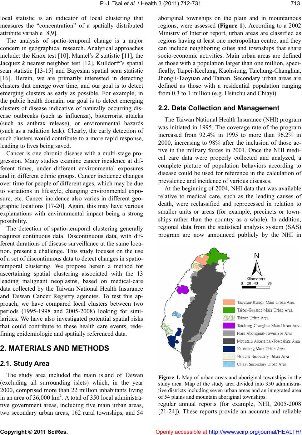

P.-J. Tsai et al. / Health 3 (2011) 712-731

713713

local statistic is an indicator of local clustering that

measures the “concentration” of a spatially distributed

attribute variable [8,9].

The analysis of spatio-temporal change is a major

concern in geographical research. Analytical approaches

include: the Knox test [10], Mantel’s Z statistic [11], the

Jacquez k nearest neighbor test [12], Kulldorff’s spatial

scan statistic [13-15] and Bayesian spatial scan statistic

[16]. Herein, we are primarily interested in detecting

clusters that emerge over time, and our goal is to detect

emerging clusters as early as possible. For example, in

the public health domain, our goal is to detect emerging

clusters of disease indicative of naturally occurring dis-

ease outbreaks (such as influenza), bioterrorist attacks

(such as anthrax release), or environmental hazards

(such as a radiation leak). Clearly, the early detection of

such clusters would contribute to a more rapid response,

leading to lives being saved.

Cancer is one chronic disease with a multi-stage pro-

gression. Many studies examine cancer incidence at dif-

ferent times, under different environmental exposures

and in different ethnic groups. Cancer incidence changes

over time for people of different ages, which may be due

to variations in lifestyle, changing environmental expo-

sure, etc. Cancer incidence also varies in different geo-

graphic locations [17-20]. Again, this may have various

explanations with environmental impact being a strong

possibility.

The detection of spatio-temporal clustering generally

requires continuous data. Discontinuous data, with dif-

ferent durations of disease surveillance at the same loca-

tion, present a challenge. This study focuses on the use

of a set of discontinuo us data to detect ch anges in spatio-

temporal clustering. We propose herein a method for

ascertaining spatial clustering associated with the 13

leading malignant neoplasms, based on medical-care

data collected by the Taiwan National Health Insurance

and Taiwan Cancer Registry agencies. To test this ap-

proach, we have compared local clusters between two

periods (1995-1998 and 2005-2008) looking for simi-

larities. We have also investigated potential spatial risks

that could contribute to these health care events, rede-

fining epidemiologic and spatially referenced data.

2. MATERIALS AND METHODS

2.1. Study Area

The study area included the main island of Taiwan

(excluding all surrounding islets) which, in the year

2000, comprised more than 22 million inhabitants living

in an area of 36 ,0 00 k m2. A total of 350 local administra-

tive government areas, including five main urban areas,

two secondary urban areas, 162 rural townships, and 54

aboriginal townships on the plain and in mountainous

regions, were assessed (Figure 1). According to a 2002

Ministry of Interior report, urban areas are classified as

regions having at least one metropo litan centre, and they

can include neighboring cities and townships that share

socio-economic activities. Main urban areas are defined

as those with a population larger than one million , speci-

fically, Taipei-K eelun g, Kaohsiung , Taich ung -Changh u a,

Jhongli-Taoyuan and Tainan. Secondary urban areas are

defined as those with a residential population ranging

from 0.3 to 1 million (e.g. Hsinchu and Chiayi).

2.2. Data Collection and Management

The Taiwan Nation al Health In suran ce (NHI) prog ram

was initiated in 1995. The coverage rate of the program

increased from 92.4% in 1995 to more than 96.2% in

2000, increasing to 98% after the inclusion of those ac-

tive in the military forces in 2001. Once the NHI medi-

cal care data were properly collected and analyzed, a

complete picture of population behaviors according to

disease could be used for reference in the calculation of

prevalence and incidence of various diseases.

At the beginning of 2004, NHI data that was available

relative to medical care, such as the leading causes of

death, were reclassified and reprocessed in relation to

smaller units or areas (for example, precincts or town-

ships rather than the country as a whole). In addition,

regional data from the statistical analysis system (SAS)

program are now announced publicly by the NHI in

Figure 1. Map of urban areas and aboriginal townships in the

study area. Map of the study area divided into 350 administra-

tive districts including seven urban areas and an integrated area

of 54 plains and mountain aboriginal townships.

regular annual reports (for example, NHI, 2005-2008

[21-24]). These reports provide an accurate and reliable

P.-J. Tsai et al. / Health 3 (2011) 712-731

714

data source for the investigation of health care issues in

Taiwan.

Data were collected from contractual medical-care in-

stitutions, where th e NHI covers the costs of prescription

medicines and treatment at outpatient clinics. Such fa-

cilities accumulate detailed databases on medical costs

for inpatient care. The number of outpatient cases were

classified in relation to disease codes, as defined in the

1975 edition of “The International Classification of Dis-

eases, 9th Revision, Clinical Modification” (ICD 9 CM).

Patients suffering from diseases that were difficult to

classify into a given code or had mismatched ID num-

bers were not included in the final statistical data set.

Disease codes were classified according to gender and

age. Cases with the same ID numbers, but which exhib-

ited different diseases, were counted as different in-

stances.

Medical care data obtained from the 2005-2008 NHI

reports were examined, and the morbidity rates of the 13

leading causes of death were calculated. Disease classi-

fications (according to the ICD 9 CM) included the fol-

lowing (indicated within parentheses): trachea, bronchus,

and lung cancer (ICD 162); liver and intrahepatic bile

ducts cancer (ICD 155); colon and rectum cancer (ICD

153, 154); stomach cancer (ICD 151); oral cavity cancer

(ICD 140, 141, 143-146, 148, 149); oesophagus cancer

(ICD 150); pancreas cancer (ICD 157); non-Hodgkin’s

lymphoma (ICD 200, 202, 203); gallbladder and extra-

hepatic bile ducts cancer (ICD 156); leukaemia (ICD

204-208); female breast cancer (ICD 174); cervix uteri

cancer (ICD 179, 180); and prostate cancer (ICD 185).

Demographic information was provided by the Minis-

try of Interior [25]. The smallest administrative units

coded for examination of the various diseases cases or

health care events were precincts and townships. Age-

adjusted standard morbidity rates, adjusted using the

Segi (“world”) population in 1976 as the standard [26],

were then calculated prov iding results giving the leading

causes of death for males and females in each township.

During the period from 1995 to 1998, data on age-

adjusted malignancies by precinct and township were

obtained from the Atlas of Cancer Mortality and Inci-

dence in Taiwan, officially published by the Bureau of

Health Promotion, Department of Health [27].

2.3. Statistics

The global Moran’s I spatial autocorrelation was used

to assess the correlation among neighbouring observa-

tions and to identify patterns and levels of spatial clus-

tering in neighbouring districts [28]. The Moran’s I sta-

tistic, similar to the Pearson correlation coefficient [29],

was calculated by the following formula:



xx x

Sxx





  (1)

where N is the number of districts, wij the element in the

spatial weight matrix corresponding to the observation

pair i, j and xi and xj observations for the areas i and j

with the mean

and:

Sij



 (2)

Since the weights were row-standardized (1





the first step in the spatial autocorrelation analysis was

to construct a spatial weight matrix that contained in-

formation about the neighbourhood structure for each

location. Adjacency was defined as immediately neigh-

boring administrative districts, including the district it-

self. Non-neighbouring administrative districts were

assigned the we i ght of zero .

Spatial contiguity for polygons is defined as the prop-

erty of sharing a common boundary or vertex. Contigu-

ity analysis is an importan t method fo r assessing unu sual

features in connectivity distribution [4,30]. The Queen’s

measure of contiguity can be utilized to make up for

spatial contiguity by incorporating both the Rook and

Bishop relationships into a single measure [30]. The

administrative districts considered in this study were

highly irregular in both shape and size. Tsai et al. (20 09)

demonstrated that the most appropriate method is the

first order queen polygon contiguity method for quanti-

fying the spatial weights matrix for the analysis of con-

nectivity. Based on this approach, the spatial weight/

connectivity matrices were determined and utilized in

conjunction with the global Moran’s I statistic and fol-

lowing LISA calculations [6].

Moran’s I va lues may range from –1 (dispersed) to +1

(clustered). A Moran’s I value of 0 suggests complete

spatial randomness. A random permutation procedure

recalculates a statistic many times by reshuffling the data

values among the map units to generate a reference dis-

tribution. The obtained calculated statistic based on the

observed spatial pattern is then compared to this refer-

ence distribution an d a pseu do significance level (pseudo

p-value) computed. To verify that the value of Moran’s I

was significantly different from the expected value, we

applied a Monte Carlo randomisation test with 999 per-

mutations to achieve highly significant values. Data

values were reassigned among the N locations, providing

a randomised distribution against which one may judge

the observed value. If the observed value of I was within

the tails of this distribution, there was significant spatial

autocorrelation in the data, a pseudo p-value smaller

than 0.05, and the assumption of independence among

the observations could be rejected [31].

LISA statistic provides information related to the lo-

P.-J. Tsai et al. / Health 3 (2011) 712-731

715715

cation of spatial clusters and outliers and the types of

spatial correlation. Local statistics are important becau se

the magnitude of spatial autocorrelation is not necessar-

ily uniform over the study area [7,32]. LISA allowed us

to divide the study area into small locations, thus ena-

bling the assessment of significant local spatial cluster-

ing around an individual location. In addition to the de-

gree of spatial clustering, detailed variations of cluster-

ing in the locally defined geo-space were identified as

well as the locations of the spatial clusters. The local

version of Moran’s I at location i is given by:





21i



ijj

wx x







 (3)

where n indicates the total number of locations (350

townships used in the years 1995-1998 and 349 town-

ships in 2005-2009); xi denotes the value of the variable

of interest, X, at location I; xj denotes the observation at

neighboring location s j; and

is th e sample average of

X. wij is the spatial weight matrix, which defines spatial

interaction across study regions. In general, wij = 1 if

location i and location j are neighboring, (share a com-

mon boundary); otherwise, wij = 0. In this study, spatial

contiguity was assessed as the first order queen’s conti-

guity which defines spatial n eighbors as those areas with

shared borders and vertexes.

Significance was tested by comparison to a reference

distribution obtained by random permutations [7]. This

analysis used 999 permutations to determine differences

between spatial un its. A positive value for the local Mo-

ran’s I index (i

) indicates that a feature has neighboring

features with similarly high or low attribute values and is

therefore part of a cluster. A negative value for (i

) in-

dicates that a feature has neighboring features with dis-

similar values; this feature is an outlier. In either instance,

the p-value for the feature must be small enough for the

cluster or outlier to be considered statistically significant.

LISA enables distinguishment between a statistically

significant (0.05 level) cluster of high values (HH), a

cluster of low values (LL), an outlier in which a high

value is surrounded primarily by low values (HL), and

an outlier in which a low value is surrounded primarily

by high va lues (LH). In add itio n to the va lue of a z-score

larger than +1.96, the outcomes are defined as clusters

with both HH and LL. In th e case of a value of a z-score

less than –1.96, the outlier is considered as clusters with

(HL) and (LH). We consider that outliers may not be

stablily and precisely displayed the outcomes of spatio-

temporal pattern comparison, because it is difficult to

distinguish between outliers how strength with or with-

out disease risks. Therefore, only hot and cold spots are

mapped on local Moran’s maps.

In addition to mapping, similarities between spatial

distribution patterns for the two periods (1995-1998 and

2005-2008) were determined using logistic regression

analysis. The binary response indicates whether there is

significant autocorrelation between administrative dis-

tricts or areas. The correlation is better (higher) if the

value of the z-score of the local Moran’s I statistic is

larger than +1.96 (clusters with hot spots and cold spots),

otherwise it is deemed to be low. The model is exp ressed

as:







PrHigher correlation

log Period

PrLower correlation











(4)

where the Period is considered an explanatory variable

in the logistic regression model and the two β valu es the

logistic regression coefficients of the model. Pr (Higher

correlation) and Pr(Lower correlation) denote the

“Higher” and “Lower” correlation probabilities, respec-

tively. In this study, two distinct precincts, the central

and west precincts in Tainan city, merged into one single

unified administrative unit in 2004. These unpaired data

were omitted and the total data from 348 townships were

tested using logistic regression.

Modeling of the logistic regression was performed

using SPSS 12. Global Moran’s I statistic and local Mo-

ran’s I statistic was calculated using Geoda (http://www.

geoda.uiuc.edu/), an open source spatial analysis system,

and visualized on LISA cluster maps using ArcMap 9.3.

3. RESULTS

Figure 2 displays the spatial clusters (hot spots and

clod spots) as obtained using LISA statistic for the top

13 leading malignant neoplasms for both males and fe-

males in Taiwan during two time periods (1995-1998

and 2005-2008).

Tab le 1 summarizes the results from global autocor-

relation statistics for the top 13 leading malignant neo-

plasms according to gender and in the two time periods

(1995-1998 and 2005-2008) in Taiwan. The results of

the global Moran’s I tests for most cases related to the

leading malignant neoplasms are statistically significant,

having a pseudo p-value smaller than 0.05, and indicated

spatial heterogeneity. However, opposing results (a pseu-

do p-value larger than 0.05) emerged in nine cases of

which are pancreas cancer for males (1995-1998), non-

Hodgkin’s lymphoma for males (1995-1998) and fe-

males (1995-1998 and 2005-2008), gallbladder and ex-

trahepatic bile ducts cancer for males (1995-1998) and

females (1995-1998 and 2005-2008), and leukemia for

males (2005-2008) and females (1995-1998), respec-

tively.

Table 2 summarizes the typology patterns, as calcu-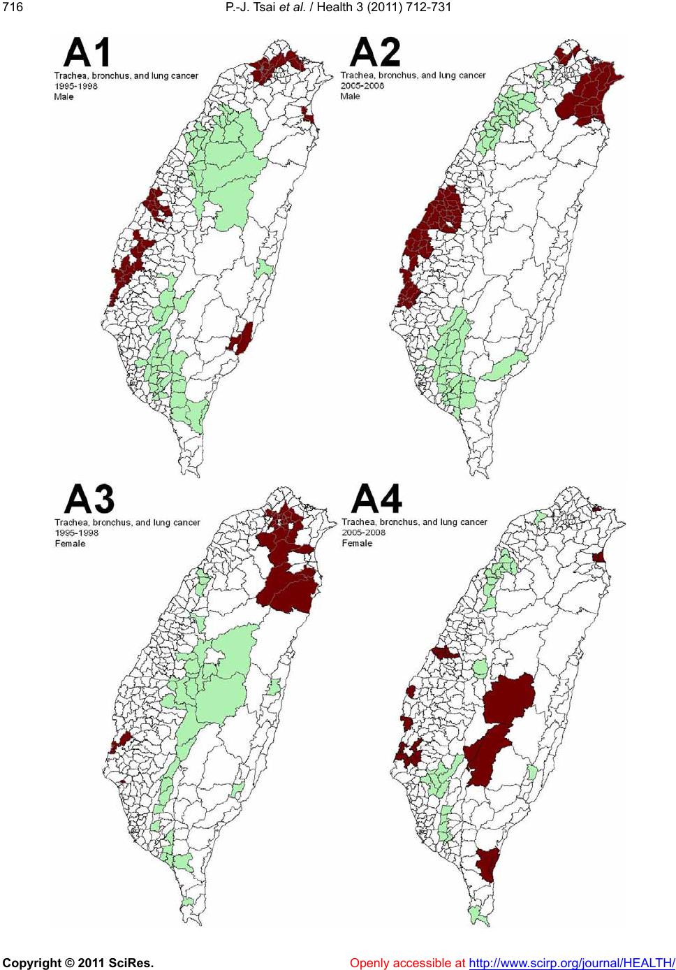

P.-J. Tsai et al. / Health 3 (2011) 712-731

716

Openly accessible at

P.-J. Tsai et al. / Health 3 (2011) 712-731

717717

P.-J. Tsai et al. / Health 3 (2011) 712-731

718

P.-J. Tsai et al. / Health 3 (2011) 712-731

719719

P.-J. Tsai et al. / Health 3 (2011) 712-731

720

P.-J. Tsai et al. / Health 3 (2011) 712-731

721721

P.-J. Tsai et al. / Health 3 (2011) 712-731

722

P.-J. Tsai et al. / Health 3 (2011) 712-731

723723

P.-J. Tsai et al. / Health 3 (2011) 712-731

724

P.-J. Tsai et al. / Health 3 (2011) 712-731

725725

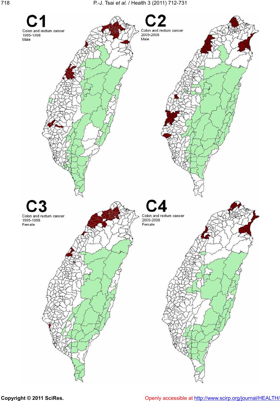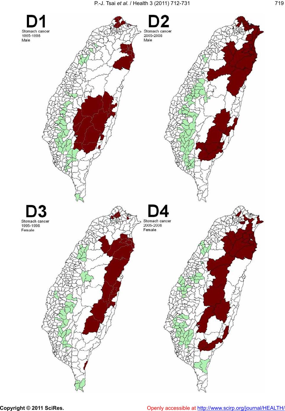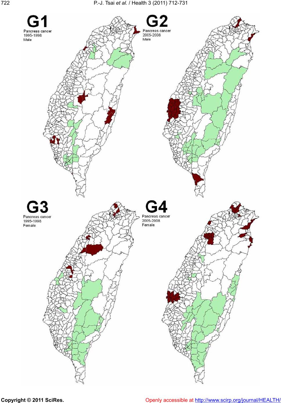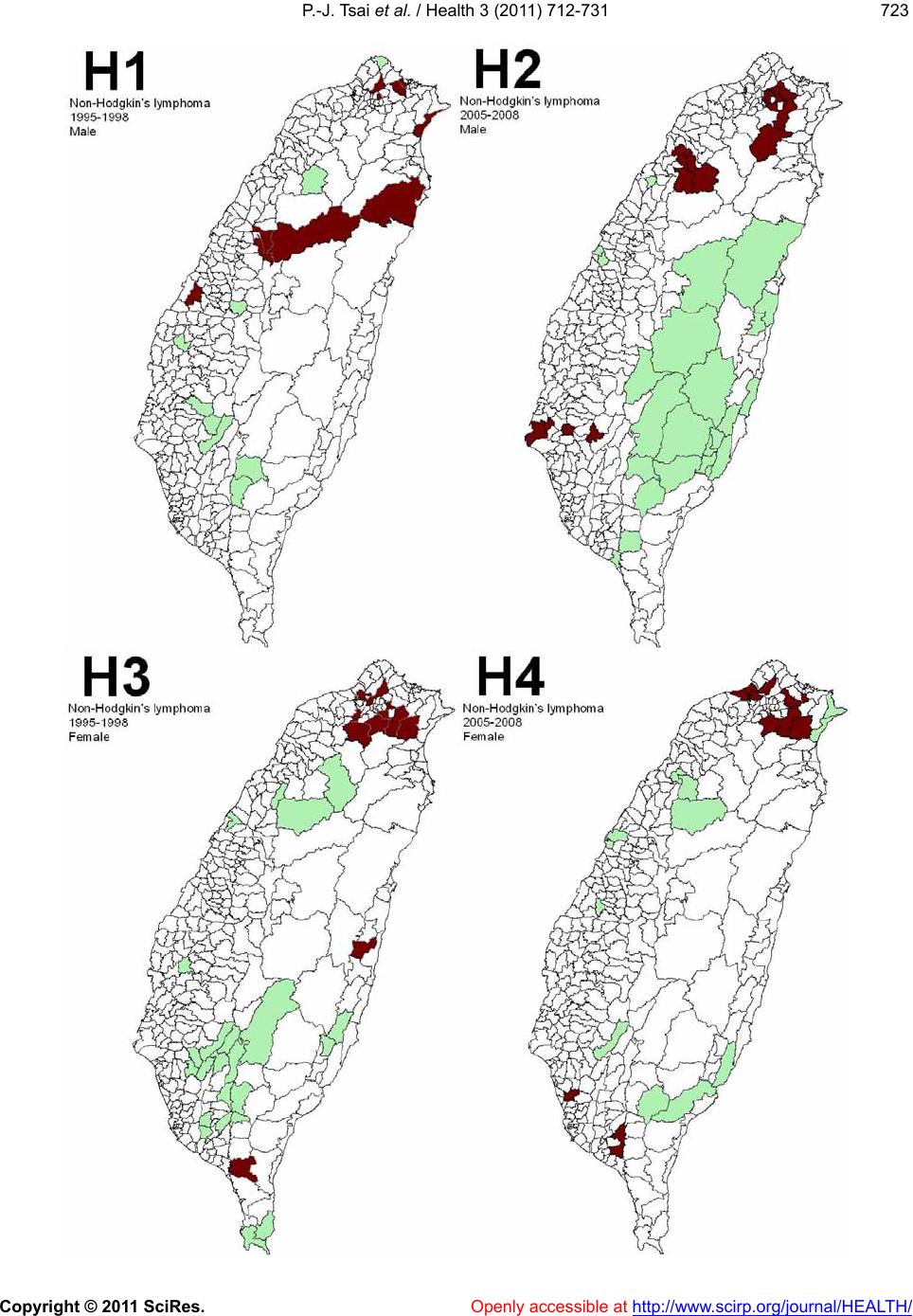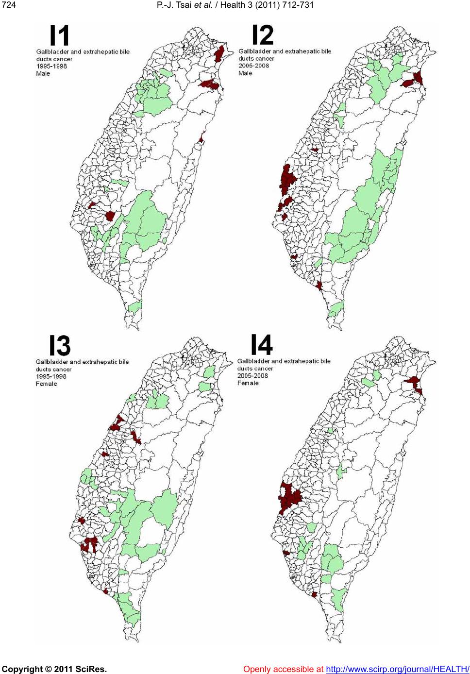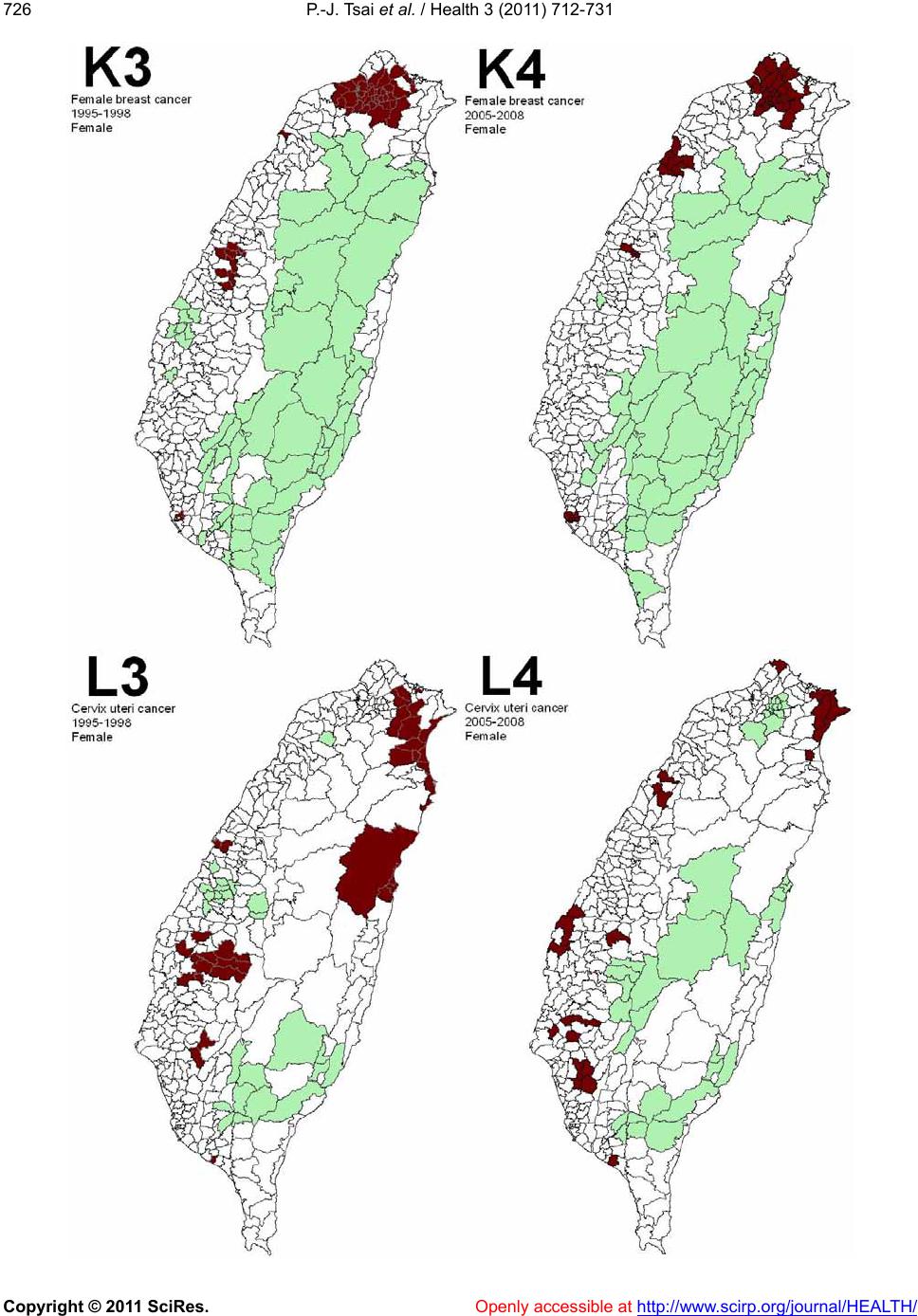P.-J. Tsai et al. / Health 3 (2011) 712-731

726

P.-J. Tsai et al. / Health 3 (2011) 712-731

727727

Figure 2. Spatial clusters of the 13 leading malignant neoplasms in Taiwan. Maps showing the spatial clusters of the 13 leading ma-

lignant neoplasms in Taiwan: A indicates trachea, bronchus, and lung cancer; B, liver and intrahepatic bile ducts cancer; C, colon and

rectum cancer; D, stomach cancer; E, oral cavity cancer; F, oesophagus cancer; G, pancreas cancer; H, non-Hodgkin’s ly mphoma; I,

gallbladder and extrahepatic bile ducts cancer; J, leukaemia; K, female breast cancer; L, cervix uteri cancer; M, prostate cancer. 1

indicates males within the period from 1995 to 1998 years; 2, males within the period from 2005 to 2008 years; 3, females within the

period from 1995 to 1998; 4, females within the period from 2005 to 2008.

lated using LISA statistic, categorized as clusters or non-

clusters at a z-score larger than +1.96. It also compares

the top 13 leading malignant neoplasms during the two

time periods (1995-1998 and 2005-2008).

Dissimilarities between the spatial distribution pat-

terns during the two periods (1995-19 98 and 2005-2 008)

are not statistically significant (p-value > 0.05) in males

for six out of eleven spatial clusters, and in females for

ten of twelve spatial clusters. In males, there are dis-

similarities for stomach cancer, oral cavity cancer, pan-

creas cancer, non-Hodgkin’s lymphoma, and prostate

cancer. In females, colon and rectum cancer, and pan-

creas cancer are dissimilar. Ta b l e 2 presents these find-

ings.

4. DISCUSSION

Locations in close proximity tend to share similar

attributes. According to Tobler (1979), “everything is

related to everything else, and nearby things are more

closely related to nearby things than to distant things”

[33]. In epidemiology, a cluster becomes apparent when

a number of health events occur which are situated close

together in space and/or time. The evaluation of spatial

distributions as a measure of disease risk may provide

etiological insights [34]. Spatial autocorrelation is the

relation between the values of a single variable attribut-

able to the geographic arrangement of areal units on a

map and can be used to determine the degree of spatial

clustering [35,36]. In this study, local Moran’s I statistic

was used to measure the degree of spatial clustering and

map the geographic patterns of the areal units. Spatial

clustering of the leading cause of death (also called hot

spots and cold spots) was identified by a z-score value

arger than +1.96. In epidemiology, “hot spots” are l

Openly accessible at

P.-J. Tsai et al. / Health 3 (2011) 712-731

728

Table 1. Global autocorrelation analysis of data for the 13 leading malignant neoplasms in Taiwan, according to gender, during 1995-

1998 and 2005-2008.

Moran’s I

Leading malignant neoplasms (ICD code) Male Female

1995-1998 2005-2008 1995-1998 2005-2008

Trachea, bronchus, and lung cancer (ICD 162) 0.38* 0.46* 0.17* 0.17*

Liver and intrahepatic bile ducts cancer (ICD 155) 0.45* 0.59* 0.34* 0.42*

Colon and rectum cancer (ICD 153, 154) 0.40* 0.52* 0.40* 0.49*

Stomach cancer (ICD 151) 0.34* 0.37* 0.22* 0.35*

Oral cavity cancer (ICD 140, 141, 143- 146, 148, 149) 0.43* 0.68* 0.09* 0.68*

Oesophagus cancer (ICD 150) 0.24* 0.22* 0.07* 0.25*

Pancreas cancer (ICD 157) 0.05 0.18* 0.07* 0.22*

Non-Hodgkin’s lymphoma (ICD 200, 202, 203) 0.02 0.07* 0.05 0.05

Gallbladder and extrahepa t i c b i l e ducts cancer (ICD 156) 0.06 0.14* 0.05 0.04

Leukaemia ( ICD 204-208) 0.08* 0.04 0.01 0.08*

Female breast cancer (ICD 174) n.d. n.d. 0.52* 0.53*

Cervix uteri cancer (ICD 179, 180) n.d. n.d. 0.24 * 0.26*

Prostate cancer (ICD 185) 0.12* 0.60* n.d. n.d.

n.d.: no detection. *: A pseudo p-value smaller than 0.05.

Table 2. Logistic regression model comparisons of the 13 leading malignant neoplasms in Taiwan, during 1995-1998 and 2005-2008.

Male Female

Leading malignant neoplasm s (I CD code) p-value description p-value description

Trachea, bro n c h u s , and lung cancer (ICD 162) 0.245 similaritya 0.21 similaritya

Liver and intrahepatic bile duc t s c anc er (ICD 155) 0.505 similaritya 0.412 similaritya

Colon and rectum cancer (ICD 153, 154) 0.492 similaritya 0.019 dissimilaritya

Stomach cancer (ICD 151) 0.034 dissimilaritya 0.053 similaritya

Oral cavity cancer (ICD 1 4 0, 141, 143-146, 148, 149) 0.007 dissimilaritya 0.229 similaritya

Oesophagus cancer (ICD 150) 0.844 similaritya 0.266 similaritya

Pancreas cancer (ICD 157) 0.029 dissimilarity 0.047 dissimilaritya

Non-Hodgkin’s lymphoma (ICD 200, 202, 203) 0.006 dissimilarity 0.179 similarity

Gallbladder and extrahepatic b i le d u ct s c a nc e r (ICD 156) 0.409 similarity 0.197 similarity

Leukaemia ( ICD 204-208) 0.137 similarity 0 .781 similarity

Female breast cancer (ICD 174) n.d. 0.182 similaritya

Cervix uteri cancer (I C D 179 , 180) n.d. 0.84 similaritya

Prostate cancer (ICD 185) 0.007 dissimilaritya n.d.

n.d.: no detection. a: A comparison of the two periods during which all of Moran’s test results are clusters (results based on Table 1).

considered interesting because of their correlation to

aetiology. This study, therefore, focuses on the spatial

locations of 13 leading malignant neoplasms. Information

about spatial location is useful for detecting risk from a

spatial point of view. A more detailed survey of these

identified “hot spots” may provide important clues on

risk factors for these diseases.

The modifiable areal unit problem (MAUP) is a phe-

nomenon whereby analysis of the same data provides

different results, grouped into different sets of areal units.

The MAUP can be subdivided into two separate effects

that usually occur simultaneously during the analysis of

aggregated data. The scale effect causes variation in

statistical results according to different levels of aggre-

gation. An association between variables, therefore, de-

pends on the sizes of the areal units of the rep orted data.

Generally, correlation increases as the size of the areal

unit increases. The zone effect describes variations in

correlation statistics caused by the regrouping of data

into different configurations, but with the same scale.

The MAUP occurs because spatial processes generating

the observed data may exist within certain scales, and for

particular areal units. These may be reflected more or

less accurately by the boundaries in use [37]. Manley et

P.-J. Tsai et al. / Health 3 (2011) 712-731

729729

al. (2006) concluded that MAUP is not really a problem,

but rather, a resource. Data at different scale levels can

enable the identification of processes operating within

different scales. It is clear that it is not possible to define

an ideal single census geography that captures all of the

processes for all variables [37]. Furthermore, the internal

composition of given areal units may not be homoge-

neous, particularly for disease distribution. Matisziw et

al. (2008) have suggested that down-scaling the spatial

structure of polygonal units could provide valuable in-

formation pertaining to the spatial distribution of disease

[38]. In this study, administrative government regions

are almost similar but not completely consistent in the

two periods (1995-1998 and 2005-2008). This was to

some degree due to the merging of the central and west

districts in Tainan city merging into one unit in 2004.

The use of only one scale to estimate spatial distribu tion

patterns, although still a cluster comparison, would be

more convenient; however, bias could be caused by

using a non-realistic spatial boundary. An ideal process

would be to calculate the spatial autocorrelation coeffi-

cients (such as the z-scores) based on realistic boundaries

(two scales for shape files that represented 350 townships

in 1995-1998 and 349 townships in 2005-2008, respec-

tively) and then omit the values of autocorrelation co-

efficients that were non-paired data from the comparison

of the two periods within the administrative regions.

The local spatial autocorrelation coefficients can be

tested for statistical significance under two rather dif-

ferent model assumptions. The first is the classical statis-

tical assumption of normality, whereb y it is assumed that

the observed value of the coefficient is the result of the

set of z-score values being independent and identically

distributed drawings from a normal distribution, implying

that variances are cons tant across the reg ion. The second

model is one of randomization, whereby the observed

pattern of the set of z-score values is assumed to be just

one realization from all possible random permutations of

the observed values across all the zones. Both models

have important weaknesses. For example, there is an

underlying population size variatio n and a lack of homo-

geneity of probabilities; however these models are

widely implemented in software packages to provide

estimates of the significance of observed results. In the

case of the randomization model, many software pack-

ages generate a set of N random permutations of the

input data, where N is us er specified. For each simulation

run, index values are computed and the set of such

values are used to provide a pseudo-probability distribu-

tion for the given problem, against which the observed

value can be compared. A z-transform of the coefficients

under normality or randomization assumptions is distri-

buted approximately as N(0, 1); hence, this may be com-

pared to percentage points of the normal distribution to

identify particularly high or low values [39]. In this

study, the comparison of databases from the two periods

(1995-1998 and 2005-2008) was addressed by the Tai-

wan Cancer Registry and the Taiwan National Health

Insurance agencies, respectively. Although the two data-

bases have a referenced value with high validity and

reliability, this case was defined with the same diagnostic

criteria (ICD 9 CM) and a world standard population in

1976 to calculate the morbidity rate. However, the esti-

mated morbidity rates derived from the two databases

cannot be directly compared with one another. Our

suggested resolution is to change the morbidity rate into

a z-transform by using a spatial autocorrelation calcula-

tion with a randomization of 999 permutations, and this

then makes two z-transform comparisons feasible. Bino-

minal variable logistic regression models were used to

distinguish spatial distribution patterns that addressed

the two periods (1 995-1998 and 2005-2008).

Z-scores for the LISA method were calculated using

the logistic regression model and results for various

leading malignant neoplasms during two periods (1995-

1998 and 2005-2008) were compared. However, the

constraint condition for spatial clustering comparison

(such as global Moran’s tested clusters on both sides) are

required to be satisfied before calculating the logistic

regression for purposes of comparison. Based on this

constraint, the results demonstrate statistically significant

differences for stomach cancer (in males), oral cavity

cancer (in males), prostate cancer (in males), colon and

rectum cancer (in females), and pancreas cancer (in

females). Another eleven compared cases were not signi-

ficantly different. The null hypothesis is, therefore,

accepted. The accepted null hypothesis results indicate

that the common spatial factor(s) may interact with both

periods.

Few previous ecological studies relate to malignant

neoplasms and their correlation to risk factors in Taiwan,

although oral cancer and stomach cancer have been

documented and are discussed briefly below. It is hoped

that this assessment of the spatial clustering of Taiwan’s

leading malignant neoplasms can contribute to the study

of spatial epidemiology.

Two separate groups identified clusters of areas

showing elevated mortality from oral cavity cancer in

females in the aboriginal townships in eastern Taiwan.

The habits of cigarette smoking, alcohol drinking and

betel nut chewing had higher prevalence in aboriginal

women in eastern Taiwan than in women in other regions

[40,41]. Chiang et al. suggested that high-risk areas of

oral cancer incidence in males closely coincided with

spatial distribution of heavy-metal pollution in soils

(such as chromium and nickel) in central Taiwan [42]. In

P.-J. Tsai et al. / Health 3 (2011) 712-731

730

this study, oral cavity cancer clusters for each gender

were calculated using the LISA statistic. Results identify

clear spatial clustering in central Taiwan, for males, and

eastern Taiwan for females, among Taiwanese aboriginal

townships. These observations, therefore, support the

results described in previous studies. However, according

to our results, the two periods (1995-1988 and 2005-

2008), show dissimilarity in the spatial distribution of

oral cavity cancer in males. Spatial risks affecting oral

cancer morbidity in males reveal space-time changes.

These findings could be interpreted as the changing

disease clusters over time, are due to the changes of

exposure cond itions to metal pollu tant and leading to the

results of a variation of virulence. Further investigation

is therefore warranted.

Several meta-analyses identified a strong and consis-

tent association between H. pylori infection and non-

cardiac gastric cancer [43-46]. The ecological study in

Taiwan suggests an association between this infection

and gastric cancer. H. pylori in fection in early childhood

may be a key issue and, it appears, a long indu ction time

is required for gastric carcinogenesis. High gastric

cancer mortality areas are clustered in the aboriginal

townships where the prevalence of H. pylori is high [40,

47]. Our results are similar to these previous studies.

Stomach cancer clusters for males and females are

located in the Taiwanese aboriginal townships, and a

new carcinogen cluster was identified in the northern

coastal region of Taiwan. This is worthy of further

investigation. However, the two periods (1995-1988 and

2005-2008) show dissimilarity in the spatial distribution

of gastric cancer in males. Spatial risks affecting gastric

cancer morbidity in males reveal space-time changes. By

changing disease clusters over time, a possible reason is

due to the changes of prevalence ranges of H. pylori or

increased in the interference of other risks in the study

area. Further investigation is therefore warranted.

5. CONCLUSIONS

A method which combines LISA statistics and log istic

regression is an effective tool for the detection of space-

time patterns with discontinuous data. Similarity is a

result of unchangeable condition in disease risks. Con-

versely, dissimilarity is deemed a significant change of

morbidity risks over the studied periods. This enables

planners to assess spatial risk factors and to determine

the most advantageous types of health care policies for

the planning and imple mentation of health care services.

These issues can greatly improve the performance and

effectiveness of health care services and also provide a

clear outline for better understanding of the results in

depth.

6. ACKNOWLEDGEMENTS

The authors would like to thank Taiwan’s Department of Health for

providing the National Health Insurance and Bureau of Health Pro mo-

tion databases.

REFERENCES

[1] Gesler, W. (1986) The uses of spatial analysis in medical

geography: A review. Social Science & Medicine, 23,

963-973. doi:10.1016/0277-9536(86)90253-4

[2] Cuzick, J. and Edwards, R. (1990) Spatial clustering for

inhomogeneous populations. Jo u rnal of the Roy al Statistical

Society, 52, 73-104.

[3] Cressie, N.A.C. (1993) Statistics for spatial data. Wiley,

New York.

[4] Legendre, P. and Legendre, L. (1998) Numerical ecology.

2nd English Edition, Elsevier , Amsterdam.

[5] Fortin, M.J. (1999) Spatial statistics in landscape ecology.

In: Klopatek, J.M. and Gardner, R.H., Eds., Landscape

Ecological Analysis: Issues and Applications, Springer-

Verlag, New York, 253-279.

doi:10.1007/978-1-4612-0529-6_12

[6] Tsai, P.J., Lin, M.L., Chu, C.M. and Perng, C.H. (2009)

Spatial autocorrelation analysis of health care hotspots in

Taiwan in 2006. BMC Public Health, 9, 464.

doi:10.1186/1471-2458-9-464

[7] Anselin, L. (1995) The local indicators of spatial associa-

tion―LISA. Geographical Anal ysis, 27, 93-115.

d oi:10.1111/j.1538-4632.1995.tb00338.x

[8] Getis, A. and Ord, J.K. (1992) The analysis of spatial

association by use of distance statistics. Geographical

Analysis, 24, 189-206.

d oi:10.1111/j.1538-4632.1992.tb00261.x

[9] Getis, A. and Ord, J.K. (1996) Local spatial statistics: An

overview. In: Longley, P. and Batty, M., Eds., Spatial

Analysis: Modeling in A GIS Environment, John Wiley &

Sons, New York, 261-277.

[10] Knox, E.G. (1964) The detection of space-time interac-

tion. Appied Statistics, 13, 25-29.

doi:10.2307/2985220

[11] Mantel, N. (1967) The detection of cancer clustering and

the generalized regression approach. Cancer Research,

27, 209-220.

[12] Jacquez, G.M. (1996) A k nearest neighbor test for

space-time interaction. Statistics in Medicine, 15, 1935-

1949.

doi:10.1002/(SICI)1097-0258(19960930)15:18<1935::AI

D-SIM406>3.0.CO;2-I

[13] Kulldorff, M. and Nagarwalla, N. (1995) Spatial disease

clusters: Detection and inference. Statistics in Medicine,

14, 799-810. doi:10.1002/sim.4780140809

[14] Kulldorff, M. (1997) A spatial scan statistic. Communi-

cation in Statistic: Theory and Methods, 26, 1481-1496.

doi:10.1080/03610929708831995

[15] Kulldorff, M. (1999) Spatial scan statistics: Models, cal-

culations, and applications. In: Glaz, J. and Balakrishnan,

N., Eds., Scan Statistics and Applications, Birkhäuser,

Boston, 303-322. doi:10.1007/978-1-4612-1578-3_14

[16] Neill, D.B., Moore, A.W. and Cooper, G.F. (2006) A

Bayesian spatial scan statistic. Advances in Neural In-

P.-J. Tsai et al. / Health 3 (2011) 712-731

731731

formation Processing Systems, 18, 1003-1010.

[17] Greenlee, R.T., Murray, T., Bolden, S. and Wingo, P.A.

(2000) Cancer statistics. A Cancer Journal for Clinicians,

50, 7-33. doi:10.3322/canjclin.50.1.7

[18] Adami, H.O., Hunter, D. and Trichopoulos, D. (2002)

Textbook of cancer epidemiology. Oxford University

Press, New York.

[19] Parkin, D.M., Whelan, S.L., Ferlay, J., Teppo, L. and

Thomas, D.B. (2002) Cancer incidence in five continents.

IARC Scientific Publications, Lyon.

[20] Frank, S.A. (2007) Dynamics of cancer: Incidence, in-

heritance, and evolution. Princeton University Press,

Princeton.

[21] National Health Insurance (2007) Statistical annual re-

port of medical care 2005. National Health Insurance

(Taiwan), Taipei.

[22] National Health Insurance (2008) Statistical annual re-

port of medical care 2006. National Health Insurance

(Taiwan), Taipei.

[23] National Health Insurance (2009) Statistical annual re-

port of medical care 2007. National Health Insurance

(Taiwan), Taipei.

[24] National Health Insurance (2010) Statistical annual re-

port of medical care 2008. National Health Insurance

(Taiwan), Taipei.

[25] Ministry of the Interior (2009) The demographic data-

base. http://www.moi.gov.tw/stat/index.aspx

[26] Ahmad, O.E., Boschi-Pinto, C., Lopez, A.D., Murray,

C.J.L., Lozano, R. and Inoue, M. (2000) Age standardi-

zation of rates: A new WHO standard (GPE discussion

paper series, No. 31). World Health Organization Press,

Geneva.

[27] Liaw, Y.P., Chen, C.J., Lee, W.C. and Hsu, S.Y. (2003)

The construction and use of the electric atlas of cancer

mortality and incidence in Taiwan. Taiwan Journal of

Public Health, 22, 227-236.

[28] Boots, B.N. and Getis, A. (1998) Point pattern analysis.

Sage Publications, Newbury Park.

[29] Cliff, A.C. and Ord, J.K. (1973) Spatial autocorrelation.

Pion Limited, London.

[30] Grubesic, T.H. (2008) Zip codes and spatial analysis:

Problems and prospects. Socio-Economic Planning Sci-

ences, 42, 129-149. doi:10.1016/j.seps.2006.09.001

[31] Cliff, A.D. and Ord, J.K. (1981) Spatial processes: Mod-

els and applications. Pion Limited, London.

[32] Ord, J.K. and Getis, A. (1995) Local spatial autocorrela-

tion statistics: Distributional issues and an application.

Geographical Analysis, 27, 286-306.

d oi:10.1111/j.1538-4632.1995.tb00912.x

[33] Tobler, W. (1979) Cellular geography. In: Gale, S. and

Olsson, G., Eds., Philosophy in Geography, Riedel, Dor-

drecht, 379-386.

[34] Moore, D.A. and Carpenter, T.E. (1999) Spatial analyti-

cal methods and geographic information systems: Use in

health research and epidemiology. Epidemiologic Re-

views, 21, 143-161.

[35] Griffith, D.A. and Arnrhein, C.G. (1991) Statistical analy-

sis for geographers. Prentice Hall, Englewood Cliffs.

[36] Kitron, U. and Kazmierczak, J.J. (1997) Spatial analysis

of the distribution of Lyme disease in Wisconsin. Ameri-

can Journal of Epidemiology, 145, 558-566.

[37] Manley, D., Flowerdew, R. and Steel, D. (2006) Scales,

levels and processes: Studying spatial patterns of British

census variables. Computers, Environment and Urban

Systems, 30, 143-160.

doi:10.1016/j.compenvurbsys.2005.08.005

[38] Matisziw, T.C., Grubesic, T.H. and Wei, H. (2008)

Downscaling spatial structure for the analysis of epide-

miological data. Computers, Environment and Urban

Systems, 32, 81-93.

[39] De Smith, M.J., Goodchild, M.F. and Longley, P.A.

(2007) Geospatial Analysis: A comprehensive guide to

principles, techniques and software tools. Matador,

Leicester.

[40] Lin, J.T., Wang, L.Y., Wang, J.T., Wang, T.H. and Chen,

C.J. (1995) Ecological study of association between

Helicobacter pylori infection and gastric cancer in Tai-

wan. Digestive Diseases and Sciences, 40, 385-388.

doi:10.1007/BF02065425

[41] Yang, Y.H., Lee, H.Y., Tnug, S. and Shieh, T.Y. (2001)

Epidemiological survey of oral submucous fibrosis and

leukoplakia in aborigines of Taiwan. Journal of Oral

Pathology & Medicine, 30, 213-219.

doi:10.1034/j.1600-0714.2001.300404.x

[42] Chiang, C.T., Hwang, Y.H., Su, C.C., Tsai, K.Y., Lian,

I.B., Yuan, T.H. and Chang, T.K. (2010) Elucidating the

underlying causes of oral cancer through spatial cluster-

ing in high-risk areas of Ta iwan with a distinct gender ra-

tio of incidence. Geospatial Health, 4, 231-242.

[43] Huang, J.Q., Sridhar, S., Chen, Y. and Hunt, R.H. (1998)

Meta-analysis of the relationship between Helicobacter

pylori seropositivity and gastric cancer. Gastroenterology,

114, 1169-1179. doi:10.1016/S0016-5085(98)70422-6

[44] Eslick, G.D., Lim, L.L. and Byles, J. (1999) Association

of Helicobacter pylori infection with gastric carcinoma:

A meta-analysis. The American Journal of Gastroen-

terology, 94, 2373-2379.

d oi:10.1111/j.1572-0241.1999.01360.x

[45] Xue, F.B., Xu, Y.Y. and Wan, Y. (2001) Association of

Helicobacter pylori infection with gastric carcinoma: A

meta-analysis. World Journal of Gastroenterology, 7,

801-804.

[46] Wang, C., Yuan, Y. and Hunt, R.H. (2007) The associa-

tion between Helicobacter pylori infection and early gas-

tric cancer: A meta-analysis. World Journal of Gastroen-

terology, 102, 1789-1798.

d oi:10.1111/j.1572-0241.2007.01335.x

[47] Teh, B.H., Lin, J.T., Pan, W.H., Lin, S.H., Wang, L.Y.,

Lee, T.K. and Chen, C.J. (1994) Seroprevalence and as-

sociated risk factors of Helicobacter pylori infection in

Taiwan. Anticancer Research, 14, 1389-1392.