Journal of Service Science and Management, 2011, 4, 440-444
doi:10.4236/jssm.2011.44049 Published Online December 2011 (http://www.SciRP.org/journal/jssm)
Dynamic Pricing of Perishable Products under
Consumer Factor*
Yanming Ge, Jianxin Zhang
1College of IT, Shanghai Ocean University, Shanghai, China.
Received September 5th, 2011; revised October 16th, 2011; accepted November 10th, 2011.
ABSTRACT
With effect of consumer factor considered, a model for dynamic pricing of perishable products is proposed. By this
model, we obtained a property of the value function: marginal value is a decreasing function of the capacity and an
increasing function of the consumer factor. Basing on this property, we proposed the following pricing strategy: ac-
cording to the regions that the perishable products are sold, we adopt the appropriate consumer factor and then use the
routine pricing strategy. This strategy not only maximizes the retailer’s revenue but also improves its service level.
Lastly, a constructive example is discussed.
Keywords: Revenue Management, Dynamic Pricing, Perishable Product, Bellman Equation
1. Introduction
Since the adoption of reform and opening-up policy,
China residents’ consumptive level has been dramatically
increasing as a whole. In the meanwhile, owin g to the di-
fference of history and culture, the consumptive level in
different regions differs greatly. Furthermore, this trend
is still upwards. Although some rules and regulations
were drawn up by Chinese government in order to ex-
pand domestic demand, the status quo is not changed but
aggravated. Under these circumstances the retailers should
take what kind of price strategies to maximize their own
revenues and respond to the call of the government (in
other word: improve the service level). I will discuss this
problem in this paper.
There are many perishable products in reality, such as:
meats, drugs, fashionable dress. Usually, perishability is
classified into two categories [1]: fixed lifetime and ran-
dom lifetime. In this paper we will restrict attention only
to the former category.
The papers related to optimal pricing for perishable
product are abundant. Gallego and van Ryzin [2] constru-
cted a continuous-time, time-homogeneous stochastic mo-
del to analyze some properties of optimal price, give an
exact solution in the exp onential demand case, and prove
the asymptotic optimality of the deterministic policy.
Bitran and Mondschein [3] analyzed a discrete-time pri-
cing model and tested in on apparel retail data. Zhao and
Zheng [4] discussed the continuous-time model with a
time-varying demand function and provided results on
the monotonicity of optimal prices over time. Das Var-
mand and Vettas [5] analyzed the problem of selling a
finite supply over an infinite horizon with discounted
revenues, where the discounting provides an incentive to
sell items sooner rather than later. Feng and Gallego [6]
discussed an interesting stochastic model of dynamic
pricing where demand is Markovian and may depend on
the current inventory level. Zhang and Cooper [7] model
a pricing control problem. They acknowledge the com-
plexity of the dynamic program, construct heuristics, and
test performance using a numerical study. Dong et al. [8]
examine both the initial inventory and subsequent dy-
namic pricing decisions with a multinomial logit model
of consumer choice. Their work focuses on horizontally
differentiated products, uses numerical experiments to
demonstrate the value of dynamic pricing, and illustrates
the value of their approach in determining near-optimal
initial inventories.
The main method used in papers [2,6,7,9] is the dy-
namic programming. There the terminal functions of op-
timality equation are usually equal to zero despite how
many produc ts are left if the salv ag e v alue is no t co nsid e-
red. We will use the same method with different terminal
*This paper is supported by program of Shanghai Ocean University (No
B-8515-10-0001) and Public welfare industry special funds research
p
rojects of The Ministry of Science and Technology of the P.R.C. (No.
200905014-06).

Dynamic Pricing of Perishable Products under Consumer Factor441
functions in this paper. In addition to obtaining the ma-
ximum revenue, our aim is to control the service level,
and it is directly reflected by the number of unsold prod-
uct at terminal time. Therefore the terminal function de-
fined in this paper adopts the following strategy: if the
number of unsold product is more than a given number,
some “penalty” will be implemented, and the poorer the
region that the stores link is, the more “penalty” is im-
plemented. The degree of “penalty” is negatively corre-
lated to a parameter, called consumer factor, which is a
function that positively correlated to the consumption
levels of the regions. Using this terminal function, the
optimality equation and some properties relating to re-
gion factors are obtained: marginal value is a decreasing
function of the capacity and an increasing function of the
consumer factor. Basing on these properties, the strategy,
which not only maximizes the retailer’s revenue but also
improves its service level, is given.
The remainder of the paper is organized as follows. In
Section 2, we describe a dynamic pricing model. In Sec-
tion 3, we investigate some properties of the expected
value function. In Section 4, we present a numerical ex-
periment to illustrate properties of the model. Conclud ing
this study, we give our conclusions in Section 5.
2. Proposed Model
2.1. Preliminaries
Consider a firm that sells
M
(discrete) items of a kind
of perishable product in Tperiods. Here we assume
there is only one customer per period and the customer in
periodt, where , has a willingness to pay
; that is, a random variable with distribution
1, 2,t

,T
t
v


,t
F
tvPv v
Therefore, if the firm offers a price in period , it
will sell exactly one unit if (with probability
p
pt
t
v

1,

F
tp). Letting

,1dtp

,Ftp
denote the demand rate, we can define an inverse-de-
mand functi o n
 


1
,1
t
ptdFdt


and revenue-rate function is
 
,,rtd dptd.
The inventory and demand in this case are both as-
sumed to be discrete. On the other hand, let
 
,,
J
td rtd
d

,
and assume it is strictly decreasing in the demand .
Equivalently, it is strictly increasing in the price . d p
Letting denote the optimal expected revenue

t
Vn
to go, if there is items of products unsold, and called
value functio n .
n
Letting


1T
Vn
 express the expected revenue at the
end of selling season (terminal time), and called terminal
function, which will be defined in the following subsec-
tion.
2.2. Definition of Terminal Function
In traditional revenue management, if salvage cost does
not consider, the expected revenue at terminal time is
defined as zero usually. It is rational because the selling
is stop at terminal time. However, if the region that is
poor, the consumption level is very low, some products
are unsold. Neither sellers nor potential customers want
to see this situation.
Here we adopt a strategy to control the number of un-
sold product, if it is more than a given number, some
“penalty” will be implemented. Firstly, let a parameter

for 01


 corresponding to the region that the
seller links, which is called consumer factor and posi-
tively correlated to the consumption level of this region,
such as: if the regions are Shanghai or Beijing,

is 1,
and

is 0.3 if they are Xining or Guiyan (they are two
cities in China). Secondly, we define a fun ction related to
the consumer factor, if the ratio of unsold product is less
than the region factor, the value of this function is zero,
otherwise is decreasing to the number of unsold product.
This is just the terminal function we want to define. For
convenience, in this paper it is defined as
  
hnAn M 

 
where
A
is a positive constant and


x
expresses the
maximum integer number less than
x
. Obviously, when
1


, the terminal function is zero, this is just the “tra-
ditional” terminal function.
2.3. Optimality Equation
In order to find the optimal policy, here we give out the
optimality equation of this prob lem, that is the following
Bellman Equation:








11
0
max ,
tt
d
Vnrtd dVnVn



t
(1)
with boundary conditions




1T
Vnhn
 and


00
t
V

for all , where
t


ttt
Vn Vn

1Vn

 is the ex-
pected marginal value of capacity.
Under the monotonic assumption of

,

J
td
*
, necessary
and sufficient condition for the optimal rate are d


1
,t

J
tdV n

 (2)
Different values of

reflect different regional con-
dition and thus, lead to distinct control policies. There-
fore, for clarity, the consumer factor parameter will ap-

Dynamic Pricing of Perishable Products under Consumer Factor
442
pear as a parameter in various notations. For example,


,
t
Vn  denotes the value function with the consumer
factor equals to

.
3. Properties of the Value Function
From Section 2, we are aware that the differences of the
value functio n, which represent the marginal revenues of
remaining capacity, play a critical role in making optimal
decisions. In this section, we explore the structural pro-
perties of the value function in Theorem 1, and another
property relating to consumer factor in Theorem 2.
Theorem 1.




,1 ,
tt
Vn Vn   .
Proof: The proof is by indu ction on .
t
First, when , from the definition of terminal
function, we have 1tT



  
 

,1 ,1
11
11
0
tt
Vn Vn
A
MnnMn
A
nMnM
other




 


 




n
It is true obviously in this case.
Assume it is true for period , and consider period
. Let denote the optimal solutio n to Bellman equa-
tion (1) for inventory level
1t
ni
t*
i
d

. From Bellman equa-
tion we have










11
**
221
**
111
**
111
**
001
,2 ,1
,2 ,1
,,
,,
,,
,,
tt
tt
t
t
t
t
Vn Vn
Vn Vn
rtdd Vn
rtdd Vn
rtdd Vn
rtdd Vn












  
 
 
 


2
1
1
1
1
1
1

1


(3)
From the optimality of , the following inequalities
hold:
*
1
d




**
111
**
221
,,
,,
t
t
rtdd Vn
rtdd Vn




 

and




**
111
**
001
,,
,,
t
t
rtdd Vn
rtdd Vn




 

Substituting into (3), rearranging and canceling terms
yields



 
*
21 1
*
01 1
,2 ,1
1,2,
,1 ,
tt
tt
tt
Vn Vn
dV nV n
dV nV n






 

 


By induction


11
,2 ,1
tt
Vn Vn 

0

 



11
,1 ,
tt
Vn Vn 

0

  

And since values at most one, and
. Therefore this conclusion is true.
d*
2
1d0
*
00d
This conclusion has intuitive implications for the op-
timal price. Note that equation (2) and Assumption
(


,
J
td is strictly increasing in the price) together p
imply that higher marginal values correspond to higher
optimal prices. Hence the more capacity remaining at any
given point in time, the lower the optimal price.
Theorem 2. If 01



 , then


,,
tt
VnVn  

Proof: The proof is by indu ction on .
t
First, when1tT

, from the definition of terminal
function, if




1MM 

, we have

 
 
 
 
 
 
 
,1 ,1
01
1
1
11
tt
Vn Vn
Mn M
An MMnM
AMnM
A
MnMn M


 



 




 



Therefore, it is true in this case. If




1MM  ,
the conclusion can be proved similarly.
Assume it is true for period and consider period
. Let 1t
t*
i
d

denote the optimal solution to Bellman equa-
tion (1) for inventory level and consumer factor is
ni

. From Bellman equation we have

 
 








11
**
111
**
001
**
111
**
001
,1 ,1
,1 ,1
,,
,,
,,
,,
tt
tt
t
t
t
t
Vn Vn
Vn Vn
rtdd Vn
rtdd Vn
rtddVn
rtdd Vn















 

1
1







(4)
From the optimality of *
1
d

and *
0
d

, the following
inequalities hold:





**
111
**
111
,,
,,
t
t
rtdd Vn
rtdd Vn






1
1


 
and





**
001
**
001
,,
,,
t
t
rtdd Vn
rtdd Vn








Substituting into (4), rearranging and canceling terms
yields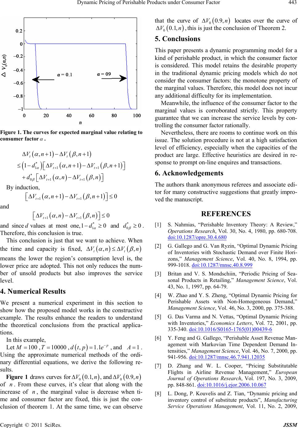

Dynamic Pricing of Perishable Products under Consumer Factor443
Figure 1. The curves for expected marginal value relating to
consumer factor

.



 
*
11 1
*
01 1
,1 ,1
1,1,
,,
tt
tt
tt
Vn Vn
dVnVn
dV nV n








 

  


1



0

By induction,
 
11
,1,1 0
tt
Vn Vn 



and
 
11
,,
tt
VnV n 

 

*
and since d values at most one, and .
Therefore, this conclusion is true. 1
10d

 *
00d 

This conclusion is just that we want to achieve. When
the time and capacity is fixed,



,,
tt
Vn Vn   
means the lower the region’s consumption level is, the
lower price are adopted. This not only reduces the num-
ber of unsold products but also improves the service
level.
4. Numerical Results
We present a numerical experiment in this section to
show how the proposed model works in the constructive
example. The results enhance the readers to understand
the theoretical conclusions from the practical applica-
tions.
In this example,
Let , , 100M10000T


,1.1
p
dtp e

, and 1
A

.
Using the approximate numerical methods of the ordi-
nary differential equations, we derive the following re-
sults.
Figure 1 draws curves for and

00.1, ,Vn



00.9,Vn
of . From these curves, it’s clear that along with the
increase of , the marginal value is decrease when ti-
me and consumer factor are fixed, this is just the con-
clusion of theorem 1. At the same time, we can observe
that the curve of
nn


00.9,Vn locates over the curve of


00.1,Vn, this is just the conclusion of Theorem 2.
5. Conclusions
This paper presents a dynamic programming model for a
kind of perishable product, in which the consumer factor
is considered. This model retains the desirable property
in the traditional dynamic pricing models which do not
consider the consumer factors: the monotone property of
the marginal values. Therefore, this model d oes not incur
any additional difficulty for its implementation.
Meanwhile, the influence of the consumer factor to the
marginal values is corroborated strictly. This property
guarantee that we can increase the service levels by con-
trolling the consumer factor rationally.
Nevertheless, there are rooms to continue work on this
issue. The solution procedure is not at a high satisfaction
level of efficiency, especially when the capacities of the
product are large. Effective heuristics are desired in re-
sponse to prompt on-line enquires and transactions .
6. Acknowledgements
The authors thank anonymous referees and associate edi-
tor for many constructive suggestion s that greatly impro-
ved the manuscript.
REFERENCES
[1] S. Nahmias, “Perishable Inventory Theory: A Review,”
Operations Research, Vol. 30, No. 4, 1980, pp. 680-708.
doi:10.1287/opre.30.4.680
[2] G. Gallego and G. Van Ryzin, “Optimal Dynamic Pricing
of Inventories with Stochastic Demand over Finite Hori-
zons,” Management Science, Vol. 40, No. 8, 1994, pp.
999-1018. doi:10.1287/mnsc.40.8.999
[3] Britan and V. S. Mondschiin, “Periodic Pricing of Sea-
sonal Products in Retailing,” Management Science, Vol.
43, No. 1, 1997, pp. 64-79.
[4] W. Zhao and Y. S. Zheng, “Optimal Dynamic Pricing for
Perishable Assets with Non-Homogeneous Demand,”
Management Science, Vol. 46, No. 3, 2000, pp. 375-388.
[5] G. Das Varma and N. Vettas, “Optimal Dynamic Pricing
with Inventories,” Economics Letters, Vol. 72, 2001, pp.
335-340. doi:10.1016/S0165-1765(01)00439-6
[6] Y. Feng and G. Gallego, “Perishable Asset Revenue Man-
agement with Markovian Time Dependent Demand In-
tensities,” Management Science, Vol. 46, No. 7, 2000, pp.
941-956. doi:10.1287/mnsc.46.7.941.12035
[7] D. Zhang and W. L. Cooper, “Pricing Substitutable
Flights in Airline Revenue Management,” European
Journal of Operations Research, Vol. 197, No. 3, 2009,
pp. 848-861. doi:10.1016/j.ejor.2006.10.067
[8] L. Dong, P. Kouvelis and Z. Tian, “Dynamic pricing and
inventory control of substitute products”, Manufacturing
Service Operations Management, Vol. 11, No. 2, 2009,

Dynamic Pricing of Perishable Products under Consumer Factor
444
pp. 317-339. doi:10.1287/msom.1080.0221
[9] Y. Akcay, H. P. Natarajan and S. H. Xu, “Joint Dynamic
Pricing of Multiple Perishable Products Under Consumer
Choice,” Management Science, Vol. 56, No. 8, 2010, pp.
1345-1361. doi:10.1287/mnsc.1100.1178