Journal of Water Resource and Protection
Vol.4 No.6(2012), Article ID:19900,7 pages DOI:10.4236/jwarp.2012.46044
Application of Artificial Neural Networks for the Prediction of Water Quality Variables in the Nile Delta
1Faculty of Engineering Mataria, Helwan University, Cairo, Egypt
2Faculty of Engineering, Fayoum University, Fayoum, Egypt
3Drainage Research Institute, National Water Research Center, Cairo, Egypt
Email: aawadallah@darcairo.com
Received March 3, 2012; revised April 2, 2012; accepted May 2, 2012
Keywords: Artificial Neural Networks; Regression with Autocorrelated Errors; Water Quality; Prediction; Nile Delta
ABSTRACT
The quality of a water body is usually characterized by sets of physical, chemical, and biological parameters, which are mutually interrelated. Since August 1997, monthly records of 33 parameters, monitored at 102 locations on the Nile Delta drainage system, are stored in a National Database operated by the Drainage Research Institute (DRI). Correlation patterns may be found between water quantity and water quality parameters at the same location, or among water quality parameters within a monitoring location or among locations. Serial correlation is also detected in water quality variables. Through the investigation of the level of information redundancy, assessment and redesign of water quality monitoring network aim to improve the overall network efficiency and cost effectiveness. In this study, the potential of the Artificial Neural Network (ANN) on simulating interrelation between water quality parameters is examined. Several ANN inputs, structures and training possibilities are assessed and the best ANN model and modeling procedure is selected. The prediction capabilities of the ANN are compared with the linear regression models with autocorrelated residuals, usually used for this purpose. It is concluded that the ANN models are more accurate than the linear regression models having the same inputs and output.
1. Introduction
Selection of variables to be sampled depends basically on the objectives and economics of monitoring. It is a highly complicated issue since there are several variables to choose from in representing surface water quality (e.g. [1]). Several methods are available. Some depended on the water uses as the main criterion, others used the level of monitoring (surveillance, intensive control, project oriented), and others applied regression methods to detect relations between water quantity and water quality variables, or between water quality variables themselves. If significant correlation is detected, then the number of variables to be observed can be reduced.
Yevjevich and Harmancioglu [2] and Harmancioglu and Yevjevich [3] investigated the transfer information by bi-variate correlations between daily observed water quality variables for the purpose of determining those variables that should be retained and need to be sampled continuously and those that can be estimated. Similar analyses were carried out by Harmancioglu et al. [4] on monthly-observed data of a highly polluted river basin. The results of these studies have shown that information transfer between water quality variables is pretty poor (e.g. [1]).
In recent years, Artificial Neural Networks (ANN) have found a number of applications in the area of water quality modeling. A good review about applications of ANNs in water quality modeling was summarised by the American Society of Civil Engineering (ASCE) task committee on application of Artificial Neural Networks in hydrology, ASCE [5]. The ASCE task committee presented different studies on water quality using the ANNs. Also, through the last few years several researchers used the ANNs in different water quality studies; Huang, and Foo [6] presented an application of the Artificial Neural Network (ANN) to assess salinity variation responding to the multiple forcing functions of freshwater input, tide, and wind in Apalachicola River, Florida. The results indicate that the ANN model is capable of correlating the non-linear time series of salinity to the multiple forcing signals of wind, tides, and freshwater input in the Apalachicola River. This study suggests that the ANN model is an easy-to-use modeling tool for engineers and water resource managers to obtain a quick preliminary assessment of salinity variation in response to the engineering modifications to the river system.
Gutiérrez-Estrada et al. [7] examined methodologies of prediction in a real-time environment for an eel intensive rearing system. Approaches based on linear multiple regression, univariate time series models (exponential smoothing and autoregressive integrated moving average (ARIMA) models) and computational neural networks (ANNs) are developed to predict the daily average ammonia concentration in rearing tanks with water recirculation. Globally, the nonlinear ANN model approach is shown to provide a better prediction of daily average ammonia concentration than do linear multiple regression and univariate time series analysis.
Water quality is influenced by many factors such as flow rate, contaminant load, medium of transport, water levels, initial conditions and other site-specific parameters. The estimation of such variables is often a complex and nonlinear problem, making it suitable for ANN application [5]. Although parametric statistical models have been the traditional approaches to detect relations between water quality parameters, many recent efforts have shown that when explicit information regression theory imposes strict conditions for error statistics, such as normal distribution and constant variance and at the same time doesn’t show encouraging results on capturing interrelation between water quality variables. Moreover, keeping in mind that ANNs are more flexible than regression models and require less prior knowledge of the system under study, it is expected that it will be a more powerful tool in capturing interrelations between water quality variables. This study aims to investigate the potential of the ANNs for modeling the relation between different water quality variables for the purpose of reducing number of variables to be observed, especially when monitoring budget is a concern. The study objective will involve the investigation of using the ANNs on estimating water quality variables, and the comparison with linear regression models with autocorrelated errors using the same inputs and outputs.
2. Methodology
In order to fulfill the objective mentioned above, the first step is to evaluate the impact of different factors that could affect the efficiency of the ANN on predicting relations between water quality variables using two different error measures. These measures will be used to select the best ANN model, as well as to compare between the ANN and the corresponding linear regression models. Data used for this study are monthly records of the Oxygen related variables, at three monitoring locations of a drainage catchment, in the Eastern Nile Delta of Egypt. Dissolved Oxygen (DO), Biological Oxygen Demand (BOD), and Chemical Oxygen Demand (COD) were measured in these locations on monthly basis from August 1997 to December 2002.
Although different factors may affect the ANN modeling, only three factors were studied in this study: the impact of using different inputs, the impact of the training vs. testing (Tr/Ts) sample sizes and combinations, and the impact of the number of nodes in the hidden layer. Besides evaluating the impact of each factor, this step is designed to select the best ANN model that will be compared with the linear regression model. Based on the fact that one hidden layer is a universal approximator [8], only one hidden layer is adopted. It was also assumed that only one or two hidden nodes are enough to capture the interrelation between inputs and output in order not to increase the number of parameters of the ANN. After several training trials, the initial weights range is fixed to be around 0.4, the learning rate is fixed at 0.1, which is the size of the steps that ANN takes toward a solution, and training is stopped at the minimum error in the testing dataset.
The COD was chosen to be the target output, which one would like to estimate using other oxygen related variables. Three different models are to be tested, the first has the BOD as a unique input (BOD model), the second has DO as a unique input (DO model), and the third model has both BOD and DO as a two-input model.
Three training/testing combinations were studied, denoted hereafter as types A, B, and C. In the type A combination, the data is divided into three equal parts, using the first two parts for training and the last part for testing (2Tr-1Ts). In the type B combination, the first part is used for testing and the last two for training (1Ts-2Tr). Finally, in the type C training testing combination, one case is used for testing and the successive two for training.
In order to evaluate the ANNs performance, two error measures are used to compare the ANNs output with observed values: Root Mean Square Error (RMSE), and Mean Absolute Relative Error (MARE). They are calculated as follows:
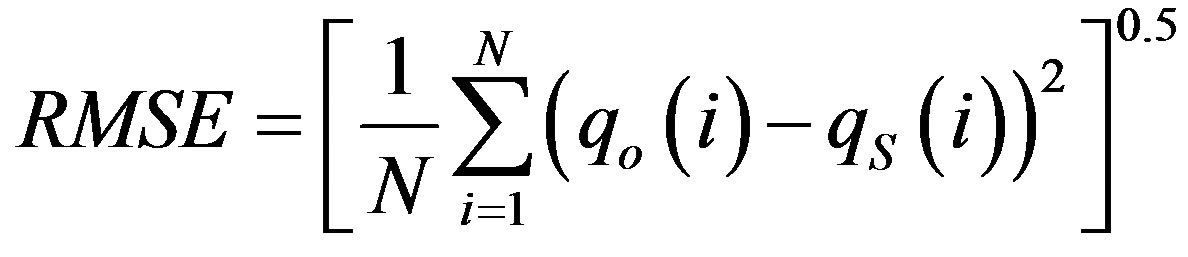 (1)
(1)
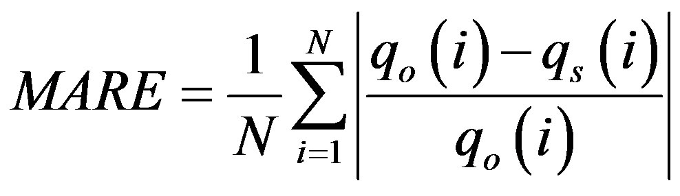 (2)
(2)
where  and
and  are the observed and predicted water quality variable at the ith observation, respectively and N is the total number of observations.
A full factorial experiment is performed to study the impact of each of the three factors explained above on the performance of the ANNs. Analysis of Variance (ANOVA) is used via the RMSE measure as the dependant variable to evaluate significance of each factor as well as the interaction among factors. The first factor is the input models. The second factor is the training testing combinations. The last factor is the number of nodes in the hidden layer. Three monitoring locations were considered in this study. Three different levels for the first two factors and two levels for the third factor will create 18 different treatments at each location.
Furthermore a sensitivity analysis is to be performed by perturbing the inputs of the selected model to test the performance of the ANN model based on the perturbation scenarios. Perturbing by +/– 10% and 20% is applied for the inputs used in the selected model.
3. Results and Discussion
3.1. ANN Simulations
The ANN simulations were performed using the BRAINCEL (ver. 4) under Excel. Total of 54 ANNs models were developed and grouped under 18 different treatments as described above. The three monitoring locations were selected to work as replicates, and not for comparison. The two error measures are tabulated for the 54 models (Tables 1 and 2). From the two tables, it is clear that the two error measures agree that the BOD model and the two-input model under the first combination using one or two nodes in the hidden layer are the best within the 18 developed models. In order to detect the significance of the impact of each factor as well as the interaction between factors, an ANOVA three-factor is performed. Table 3 shows the ANOVA table for the three investigated factors. As previously mentioned, the RMSE measure is used for ANOVA.
The ANOVA showed that interactions have no effect on the calculated RMSE. It shows also that choosing one or two nodes in the hidden layer is not significantly different. However, a significant difference is detected between the three models with different inputs, as well as for the three different Tr/Ts types. Since there is no significant difference between using one or two nodes in the hidden layer, one node hidden layer models were selected for further analysis. Selection is based on the absence of significance as showed by the ANOVA, and also to make ANN models as simple as possible to be comparable with linear regression analysis.
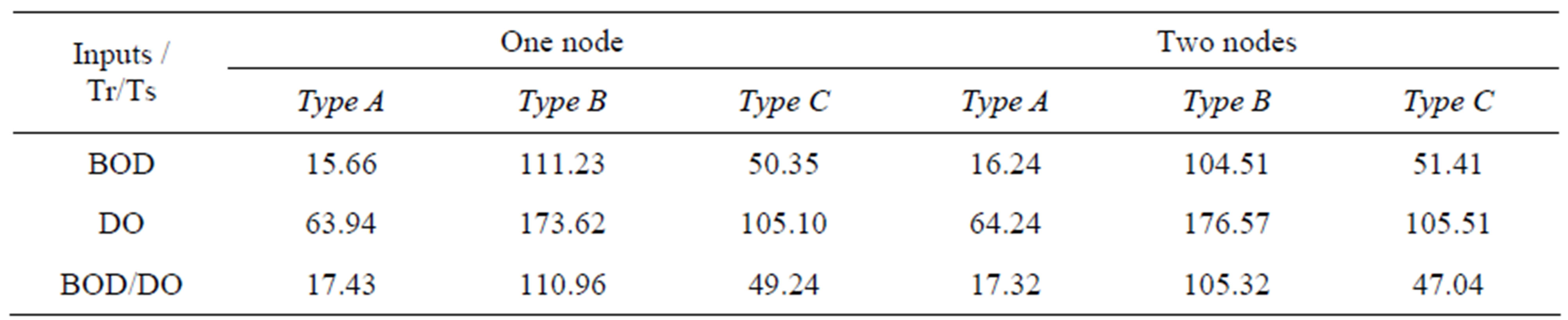
Table 1. RMSE (mg/l) measures for ANN models.

Table 2. MARE measures for ANN models.
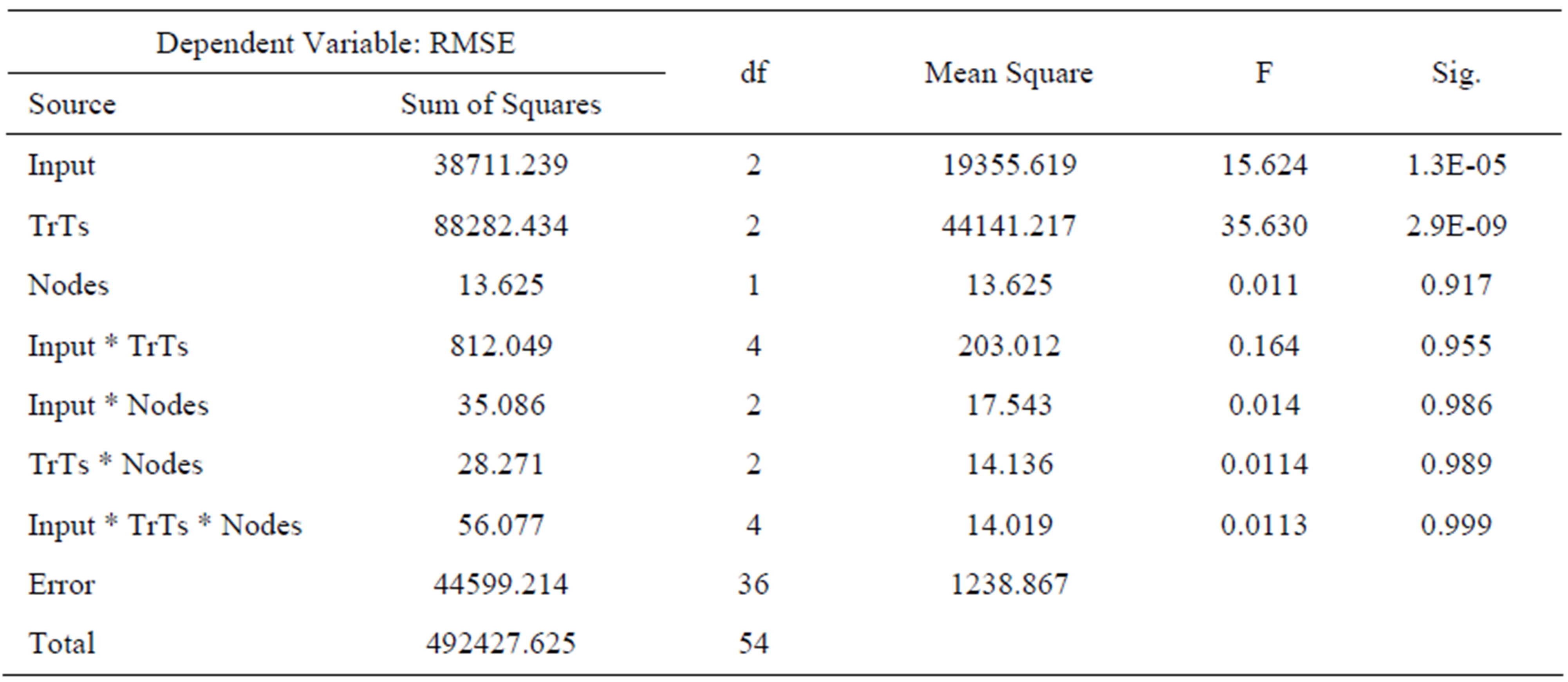
Table 3. ANOVA three factor (RMSE).
Figure 1 shows the RMSE calculated for model outputs using different inputs and different Tr/Ts combinations. It indicates that using BOD model is the best within the three models. However using the two-input model is not significantly different, while the DO model is always the worst. As for the different Tr/Ts combinations proposed, combination of type A shows the best results, while the type B combination shows the worst, and the type C combination is in-between. To show the difference between the three input models, a correlation matrix is performed using the raw data. The correlation matrices for the three monitoring locations are presented in Table 4.
From Table 4 it is obvious that COD is highly correlated with the BOD, while it is not that much correlated with DO. This is common behaviour in the three monitoring locations, so one can say that correlation with the target group is the dominant factor in choosing inputs. This lack of correlation of DO with COD could be explained by the small variation in DO values, which varied between (2 - 4 mg/l), while BOD and COD varied in a wider range. The high organic loads prevent self purification capabilities of the drains and thus keeps DO at very low levels. High correlations between COD and BOD explain why the BOD models and the two-input models are always better with respect to error measures.
To explain the impact of the Tr/Ts combination, the raw data statistical parameters were calculated using the same combination, training set and testing set of data are presented in Table 5. From Table 5, it is clear that the type A combination has a training set standard deviation double that of the testing set. While as type B has a training standard deviation half that of the testing set. As for Type C, it has almost not only the same standard deviation but also equal means between training data sets and testing sets.
The training and testing RMSE’s are presented in Figure 2 for the different input models as well as for the three types of the Tr/Ts combinations. From Figure 2 and Table 5, it is clear that significant differences appear between the training error and the testing error in the first two combinations Types A and B, while difference is not important when using Type C combination. When the variability in the training set is much bigger than that in the testing set of data, the testing error is significantly smaller than that of training, and vice versa. While using training and testing set of data which have almost the same variance or in other words coming from the same population, there will not be a significant difference between the training and testing error measures. For the purpose of inference one can trust the last combination model, which will give reliable error estimates.
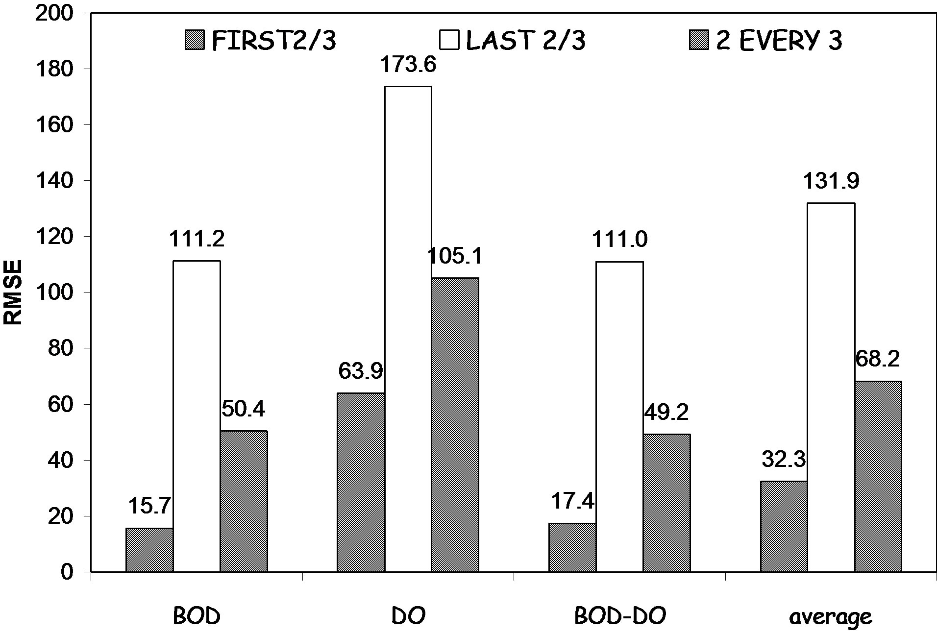
Figure 1. RMSE (mg/l) for different scenarios using one node.
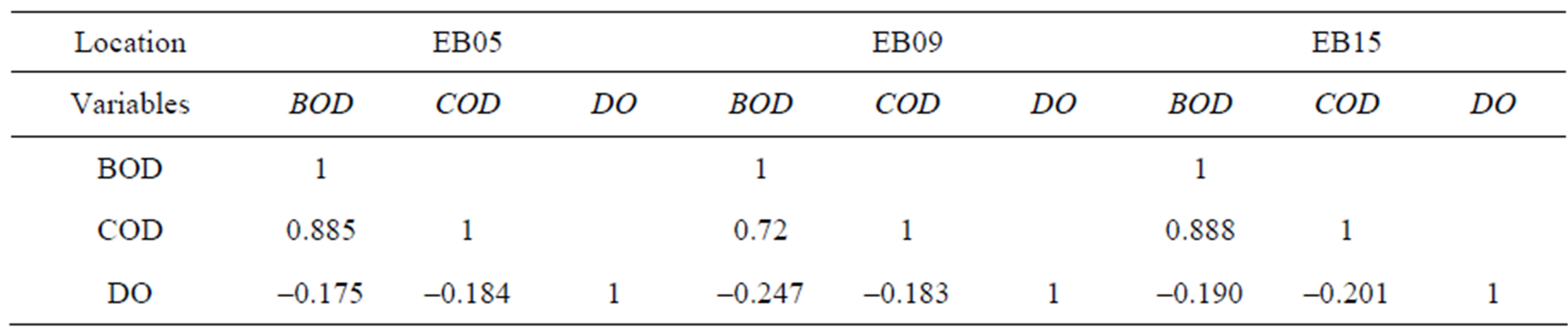
Table 4. Raw data correlation matrix.
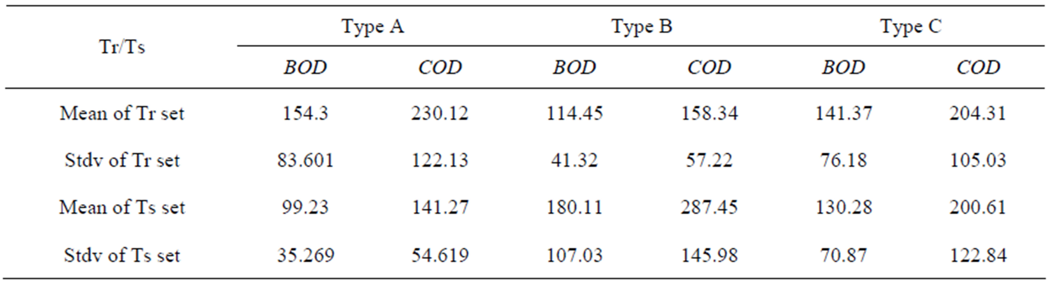
Table 5. Descriptive statistics for Tr/Ts groups.
From this analysis, one can conclude that the BOD model and the two-input model are the best, when using the Type A combination. However, the Type C results will be included in the comparison with linear regression analysis. Figure 3 shows the COD concentrations observed and predicted using the ANN at one of the locations under study (EBO5). In Figure 3, arrows indicate the data range, which may be an indicator of data variation used for training or testing. The variability of the training set is illustrated in a solid (green) arrow, while the variability in the testing set is shown in dashed (brown) arrow. Figure 3 shows also the grouping pattern of testing and training. This grouping pattern is not possible to illustrate visually for Type C.
Training the ANN using data with high variability, while testing the model on lower variability data leads to decrease the error measured on testing data (Type A). While Type C shows training and testing data sets almost from the same population; that is why there is no significant difference between training and testing errors measured using Type C combination method.
3.2. Regression Analysis
The regression analysis was performed using the SPSS 13 under windows. Linear regression models were developed for the different input types, using the three different monitoring locations records available. As the errors are correlated, as detected by the Durbin Watson statistic calculated, an ARMA model was fitted to the residuals. For the three types of models, an ARMA (1,1) model was the best suited model for the residuals. The ARMA parameters were estimated along with the coefficients of regression in the same Maximum Likelihood estimation procedure. It is worth mentioning that the coefficient corresponding to DO variable is always nonsignificant whether in the DO model or in the Two-input model. Therefore, the Do model and the two-input model are not listed in Table 6. To allow the comparison with ANN models, the same combination of type A is used; i.e. the first 2/3 of the dataset is used for regression models parameter estimation, while the last 1/3 of the dataset is used for regression model testing. Table 6 shows the error measures for both parameter estimation (training) and verification datasets. In the same Table 6, the results of several ARIMA models using only COD variable are also shown to assess the impact of the inclusion of an exogenous variable such as the DO.
Table 6 shows that using the BOD model has an average RMSE of 53 mg/l, which gives a lower RMSE than the Autoregressive models. Thus, the sole information in the COD variable is not enough to predict its behaviour and one needs to incorporate the BOD as an exogenous variable. It is worth noting that the AR(1) model is not capable to predict the decay in the COD, that’s why the RMSE in the testing set is higher than that in the training (parameter estimation) set. The ARIMA (1,1,0) is a much better predictor, but far less than the BOD model
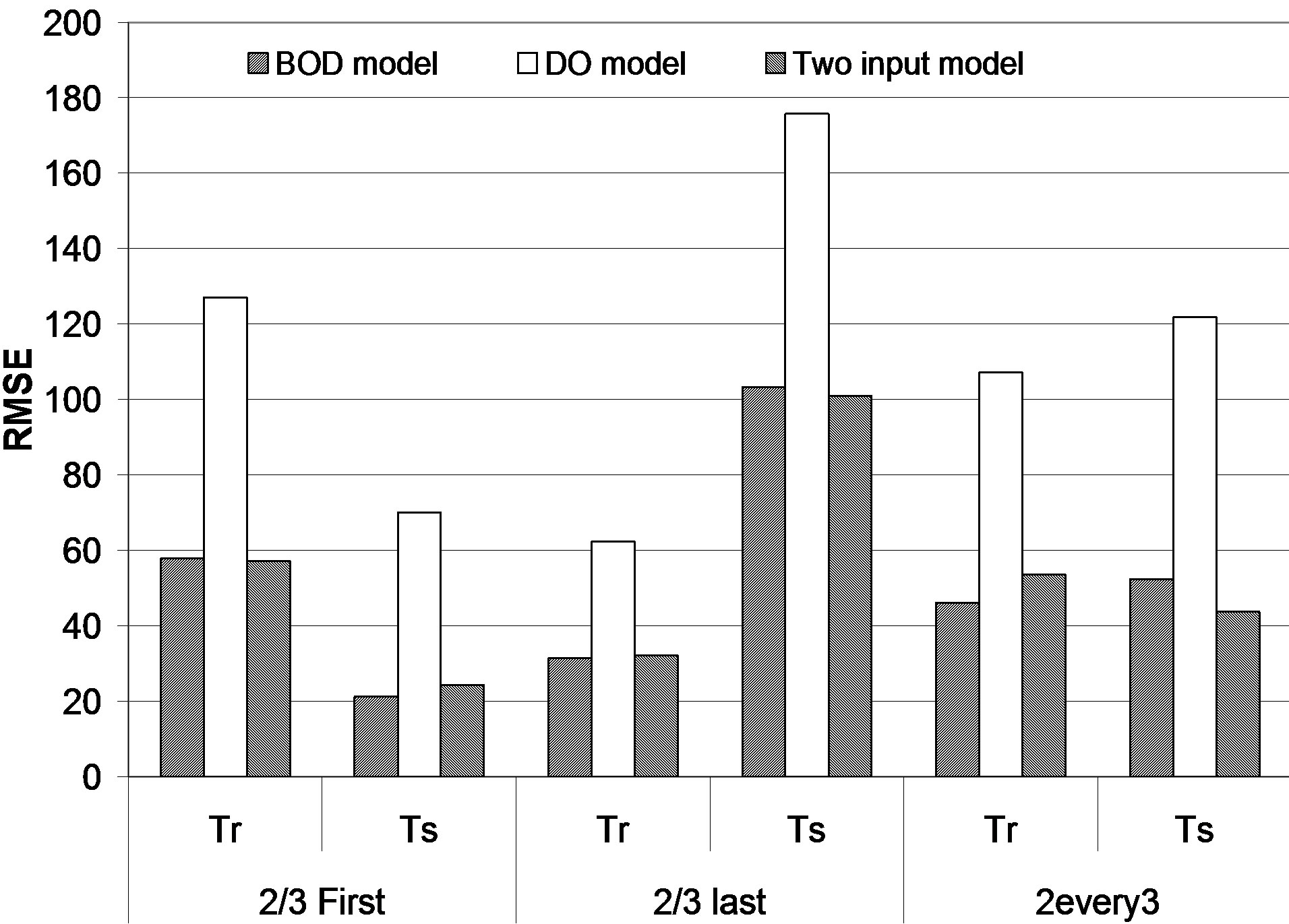
Figure 2. Training and testing RMSE (mg/l) for models using one node.
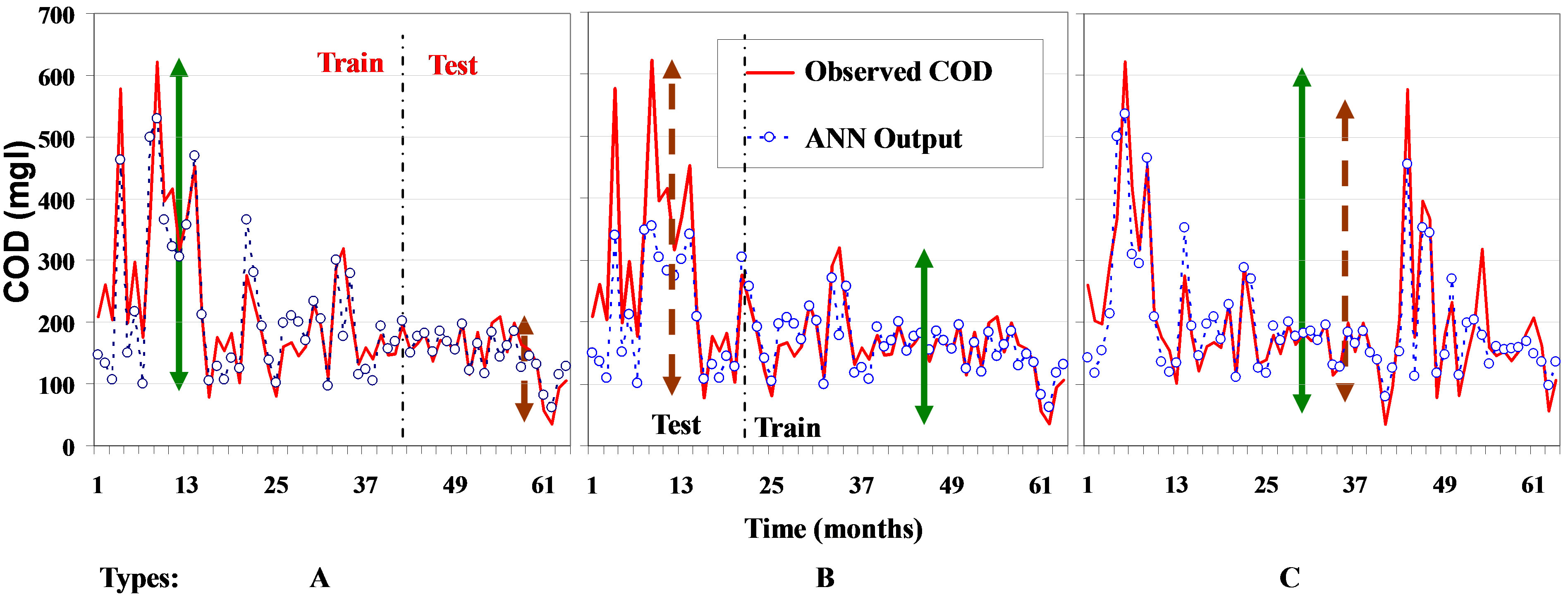
Figure 3. COD concentrations from the BOD model at EB05 (Three Tr/Ts combination).
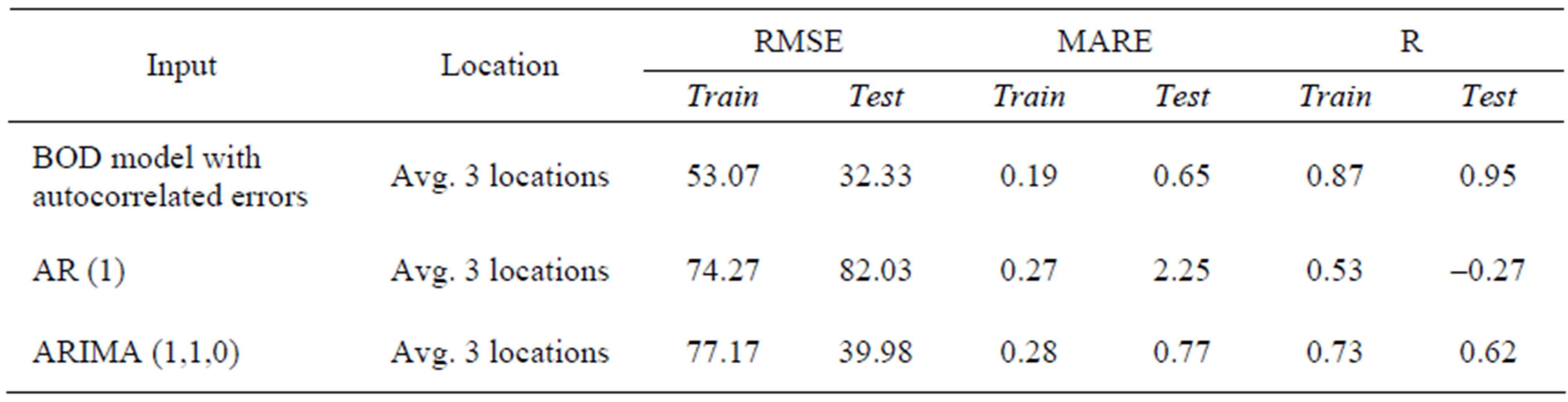
Table 6. Linear regression model error measures.
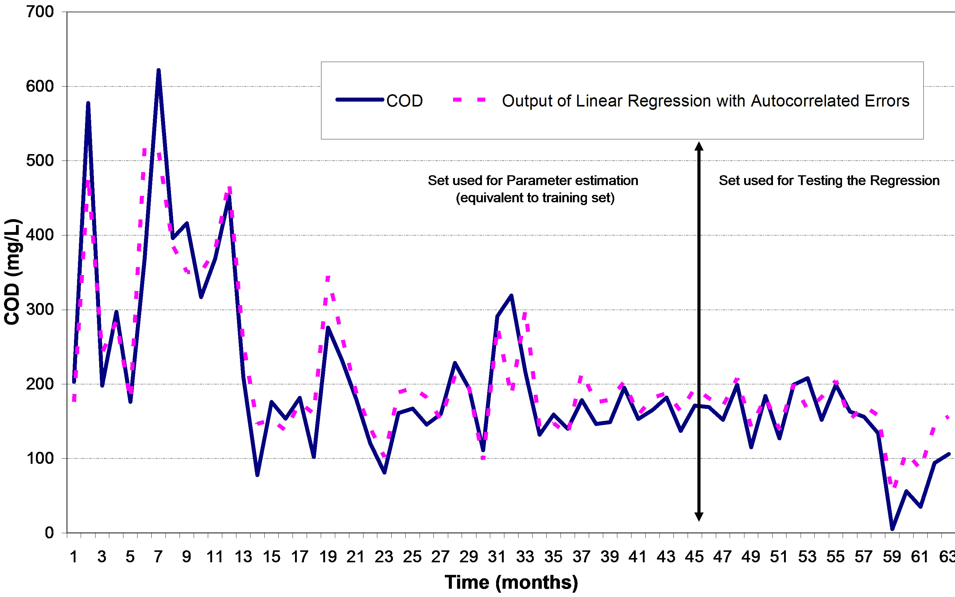
Figure 4. BOD model at EB05 (Linear regression).
with autocorrelated errors. Figure 4 shows the predicted COD concentrations versus the observed set at EB05 indicating some errors on predicting large COD concentration values in the parameter estimation set much more than on small values. The RMSE of the regression models is higher than the ANN models selected having the same inputs and output and with the same combination of Tr/Ts.
4. Sensitivity Analysis
Sensitivity analysis aims to test what happens to the performance of the ANNs models if the BOD values differ if adding up to +/– 20% perturbation on the variable. The perturbation performed used types A and C Tr/Ts combinations. Figure 5" target="_self"> Figure 5 shows the different RMSE calculated for variations of BOD concentrations by +/– 10% and 20% using the Type A or C combinations respectively.
RMSE calculated using perturbed BOD concentration is comparable to the training error (RMSE) when using type A training testing combination, while for the third combination it is comparable with the testing error. The reason may be, as mentioned before, that in the first Tr/Ts combination, the model is trained on a data set from the same population as the data set perturbed. While using the type C combination, the training, testing and perturbing errors are all close to each other. The perturbation of BOD concentrations by 10% affected the ANNs output by about 1% to 7% of the RMSE measured for testing data set error using the type C combination. The EB09 shows high variability and different behaviour than others. It reaches 30% when using the type A combination. This could be explained by the relatively lower correlation between BOD and COD for EB09 location.
5. Conclusions
In this study, the potential of the Artificial Neural Networks (ANN) on predicting interrelation between water quality parameters was examined. Several ANN inputs, structures and training possibilities are assessed and compared with linear regression models with autocorrelated errors. The results of the ANN modeling shades light on the usefulness of ANN application in the prediction of water quality variables.
Using one or two nodes in the unique hidden layer
 (a)
(a)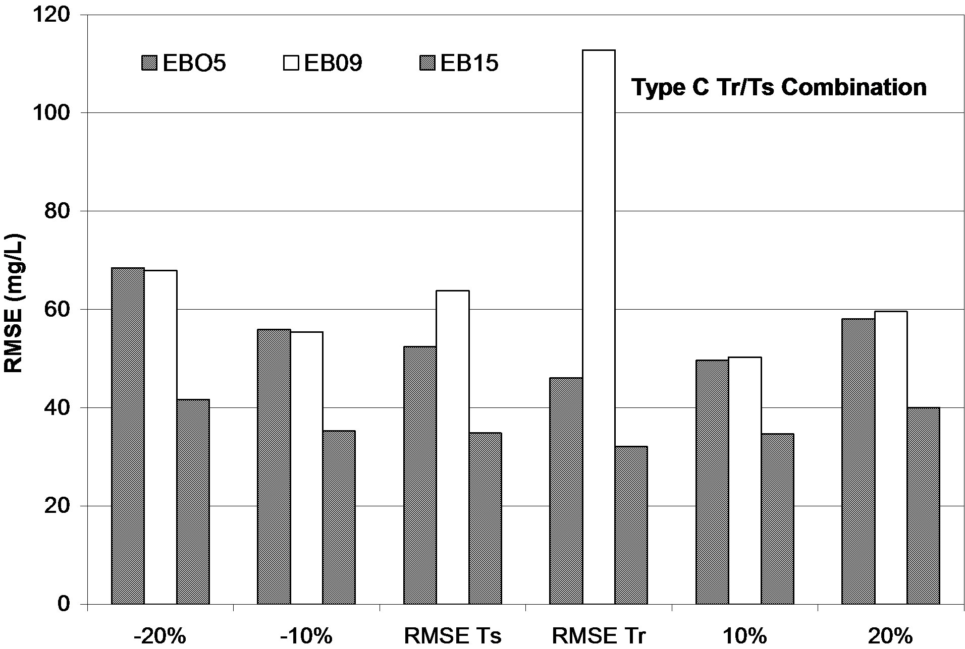 (b)
(b)
Figure 5. RMSE for BOD sensitivity analysis, (a) Type A and (b) Type C.
doesn’t affect the performance of the ANNs; for simplicity the one node layer was chosen. Analysis indicated that the linear correlation between the inputs and the target group is the dominant parameter in selecting the inputs. Using the BOD concentrations as a unique input to estimate COD concentrations in this study has the least errors measured compared to other models.
Training vs. testing combinations showed a significant effect on the performance of the ANNs, i.e. the selection of the data to be trained and that to be tested has a significant impact on the calculated errors. However, using any of the Tr/Ts combinations, the analysis indicated that during testing stages, the ANNs models were more accurate than the best linear regression model with autocorrelated errors. It is concluded that reasonably accurate monthly COD concentration predictions can be achieved using simple ANNs.
Sensitivity analysis was performed by perturbing the BOD variable. It shows that the output is sensitive to random changes of BOD concentrations. The error increase reaches 30% when the BOD concentrations is changed by 20%, while it reaches only 7% when the BOD concentrations changed by 10%.
REFERENCES
- N. B. Harmancioglu, O. Fistikoglu, S. D. Ozkul, V. P. Singh and M. N. Alpaslan, “Water Quality Monitoring Network Design,” Water Science and Technology Library, Vol. 33, Kluwer Academic Publisher, Dordrecht, 1999, pp. 187-203.
- V. Yevjevich and N. B. Harmancioglu, “Modeling Water Quality Variables of Potomac River at the Entrance to Its Estuary, Phase II (Correlation of Water Quality Variables within the Framework of Structural Analysis),” D.C. Water Resources Research Center of the University of the District of Columbia, Washington DC, 1985, 59 p.
- N. B. Harmancioglu and V. Yevjevich, “Transfer of Information among Water Quality Variables of the Potomac River, Phase III: Transferable and Transferred Information,” D.C. Water Resources Research Center of the University of the District of Columbia, Washington DC, 1986, 81 p.
- N. B. Harmancioglu, A. Ozer and N. Alpaslan, “Procurement of Water Quality Information (in Turkish). IX. Technical Congress of Civil Engineering,” Proceedings of the Turkish Society of Civil Engineers, Vol. II, 1987, pp. 113-129.
- ASCE Task Committee on Application of Artificial Neural Networks in Hydrology, “Artificial Neural Networks in Hydrology (II): Hydrologic Applications,” Journal of Hydrologic Engineering, Vol. 5, No. 2, 2000, pp. 124- 137.
- W. Huang and S. Foo, “Neural Network Modeling of Salinity Variation in Apalachicola River,” Water Research, Vol. 36, No. 1, 2002, pp. 356-362. doi:10.1016/S0043-1354(01)00195-6
- J. C. Gutiérrez-Estrada, E. De Pedro-Sanz, R. LópezLuque and I. Pulido-Calvo, “Comparison between Traditional Methods and Artificial Neural Networks for Ammonia Concentration Forecasting in an Eel (Anguilla anguilla L.) Intensive Rearing System,” Aquacultural Engineering, Vol. 31, No. 3-4, 2004, pp. 183-203. doi:10.1016/j.aquaeng.2004.03.001
- K. Hornik, “Some new results on neural network approximation,” Neural Networks, Vol. 6, No. 8, 1993, 1069- 1072. doi:10.1016/S0893-6080(09)80018-X