Journal of Water Resource and Protection
Vol. 1 No. 6 (2009) , Article ID: 1078 , 8 pages DOI:10.4236/jwarp.2009.16054
Stochastic Modelling of Actual Black Gram Evapotranspiration
1Department of Agricultural Engineering, North Eastern Regional Institute of Science & Technology, Nirjuli, India
2Department of Soil and Water Engg., CAEPHT, CAU Gangtok
3Department of Soil and Water Engg., CTAE, M.P.U.A.&T Udaipur
E-mail: pandeypk@gmail.com
Received August 29, 2009; revised September 15, 2009; accepted September 24, 2009
Keywords: Black gram (Vigna Mungo L.) Evapotranspiration, Crop water requirement, Stochastic Modelling
ABSTRACT
The study was undertaken to develop and evaluate evapotranspiration model for black gram (Vigna Mungo L.) crop under climatic conditions of Udaipur, India. Pan evaporation data for the duration of twenty three years (1978-2001) and measured black gram evapotranspiration data by electronic lysimeter for duration of kharif season of 2001 were used for analysis. Black gram is an important crop of Udaipur region. No systematic study on modelling of black gram evapotranspiration was conducted in past under above said climatic conditions. Therefore, stochastic model was developed for the estimation of daily black gram evapotranspiration using 24 years data. Validation of the developed models was done by the comparison of the estimated values with the measured values. The developed stochastic model for black gram evapotranspiration was found to predict the daily black gram evapotranspiration very accurately.
1. Introduction
The arid regions of India cover an area of 317,090 km2and lies between 240-290 N latitude and 700-760 E longitude. The region is spread over seven states, viz., Rajasthan, Gujarat, Punjab, Harayana, Maharashtra, Karanataka and Andhra Pradesh, the north-western part of the country constituting almost 90% of the total arid zone area. However, Rajasthan state alone accounts for 60% of the arid zone of India. The mean annual rainfall varies from 100 mm in the northwest to 450 mm in the eastern part of Rajasthan. The mean minimum and maximum temperature ranges from 160C to 400C. The potential evapotranspiration during summer is 7 to 9 mm/day, monsoon 5.3 to 6.4 mm/day and in winter 1.8 to 2.9 mm/ day. Thus, the evapotranspiration far exceeds precipitation throughout most of the year. The present study underlines the importance of black gram as a pulse crop on the backdrop of scarcity rainfall in the arids of Rajasthan.
Mathematical models in hydrology are suitable abstraction of complex physical phenomena. The second order model approach is of major value in the construction of mathematical models of hydrologic time series. Observed data are treated directly to produce efficient estimates of spectral representation (variance spectral) or moment functions (correlograms) of stochastic process.
Evapotranspiration process is stochastic in nature. Usually, the deterministic models do not consider the random effects and may not represent the evapotranspiration quite accurately. On the other hand, the stochastic models are based on the time dependent variations and consider random effects involved in the process. Stochastic models explain the extent of dependence of a present observation on the past observations.
A stochastic model is the mathematical abstraction of an empirical process and is governed by probabilistic laws [1].
Stochastic processes deal with continuous or discrete state and time parameters. The analysis of time series is done to understand the mechanism that generate the data and to produce likely future sequences if required. Time series are considered as a part of stochastic process.
The purpose of the stochastic model is to represent important statistical properties of one or more time series. Indeed, different types of stochastic models often studied in turns of statistical time series they generate. Models formulated on the stochastic concept explain the extent of dependence of the present observations on the past observations.
The first step in stochastic model construction is to select suitable classes or families of model from which the most appropriate model to a given time series can be chosen by following the identification, estimation and diagnostic check stages of model development. For example, when modelling a hydrologic time series one may wish to consider the Auto Regressive Moving Average (ARMA) family of models (Box and Jenkins, 1976), the classes of non Gaussian models suggested by [2] and fractional differencing models [3].
Stochastic processes deal with continuous or discrete state and time parameters. Discrete series occur when the random variate in the time series is continuous but for computation and analysis purpose time is considered discrete. A stationary series may be modelled by short memory models and non-stationary series by long memory models. Short memory models of hydrologic phenomena include moving average (MA) models, autoregressive (AR) models, and autoregressive integrated moving average (ARIMA) models. Autoregressive model (AR) has been used extensively in hydrologic analysis.
Thus,
Zt - μ = at + Ф1 (Zt-1- μ)
+ Ф2 (Zt-2. - μ) +……+ Фp (Zt-p. - μ) (1)
where
Z t = deviation from mean
μ = sample mean
Ф =autoregressive model parameters
p= order of moving average
Most of the recent advances in time series analysis are systematically discussed by [4].Comprehensive discussions on time series modelling of hydrologic variables given by [5]. Stochastic models were used extensively for forecasting of stream flow data [6]. However, the use for modelling of evapotranspiration appears to be very limited. So there is a scope of exploring the possibility of stochastic modelling of evapotranspiration. [7] developed the stochastic series of the weekly evaporation data of the Palanpur, Himachal Pradesh. [8] developed a stochastic model for the weekly evaporation and daily wheat, green gram evapotranspiration values using 20 years data under the climatic conditions of Udaipur. Validation of the developed model was done by comparison of estimated values with measured values. [9] developed a stochastic model for estimation of daily maize evapotranspiration using 23 years data under climatic conditions of Udaipur.Evapotranspiration is a basic component of hydrological cycle. Modelling of evapotranspiration process is essential for determining of appropriate model in a particular climatic condition. Therefore, stochastic modelling of Black gram evapotranspiration may provide good insight and understanding of the processes for useful applications in water resources development.
2. Material and Methods
2.1. Location of the Study Area
The study was conducted at the College of Technology and Engineering (CTAE), Udaipur. The area comes under the sub humid region of agro-climatic zone IV A of the state of Rajasthan and is situated at 24035’ N Latitude 730 42’E Longitude and at an altitude of 582.17m above mean sea level. The annual rainfall in the region is 662.5mm and more than 80% of this amount is received as a part of south – west monsoon during the period of 16th June to 15th September.
2.2. Soil of the Study Area
Relative proportion of, sand, silt and clay were found to be about 51.4, 17.5, and 31.1 per cent respectively. As per USDA, soil is classified as sandy loam. Values of bulk density of soil at depth 0-30 cm and below 30 cms were found to be 1.57 and 1.62 g/cc respectively. Average rate of infiltration is about 2.2 cm/hr. Field capacity and permanent wilting point were found to be 21.0 and 6.0 percent respectively on dry weight basis. Average electrical conductivity (EC) of the soil samples was found to be 0.18 dS/m at 250C. Soil is alkaline in nature having pH 8.2.
2.3. Collection of Evaporation and Metrological Data
The data of pan evaporation, air temperature, relative humidity, wind speed, sunshine hours, for a period of twenty-four years (1978-2001) were collected from Meteorological Observatory of the College of Technology and Engineering, Udaipur.
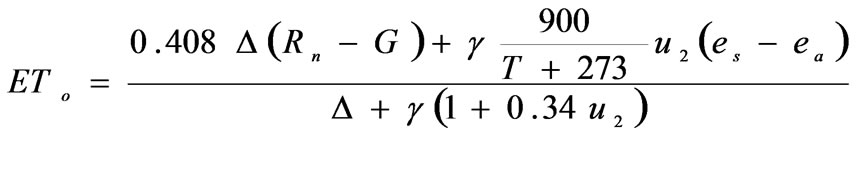
The reference evapotranspiration (ET0) was calculated by the following Penman-Monteith FAO-56 equation [10]:
2.4. Measurement of Evapotranspiration for Black Gram Crop
An electronic weighing lysimeter consisting of two steel tanks of size 1.17 m x 1.47 m for the inner and 1.23 m x 1.53 m for the outer tanks was used for this study. A pit of 1.5 m x 1.75 m x 1.75 m was made for the installation of outer tank. The bottom of the pit was well compacted. A stone soling was constructed and then a 30.0 cm thick layer of cement concrete was laid. After proper curing for about 15 days the outer tank was rested on the cement platform in such a manner so that the rim of the tank was 10.0 cm above the soil surface. The inner tank was rested on the four load cells fitted on the corner of the outer tank. Data logger was fitted in the data acquisition almirah at 50.0 m away from the lysimeter.
The weighing arrangement was made with the help of load cells and data logger. When positioned, the gap between the inner and outer tank was kept uniform. A layer of 15 cm gravel and 15 cm sand was laid on the bottom of inner tank. Backfilling of the inner tank was made in layers of 15 cm soil. When filled with soil, all the four load cells were calibrated. A drainpipe was installed at the corner of the inner tank. This pipe was covered with synthetic filter. The weighing lysimeter can read correctly up to 500.0 gm. The least count of the measurement of lysimeter is 0.28 mm.
Black gram crop of variety T- 9 was grown from 19th July 2001 to 8th October 2001 for measurement of daily evapotranspiration. The row-to-row spacing was kept 30 cm and plant to plant spacing was kept 15 cm. The seed of black gram was placed 5 cm below the soil surface. The seed rate was taken as 15 kg per hectare. All the agronomical practices were done in accordance with the standard recommendations.
2.5. Formulation of Stochastic Model for Black Gram Evapotranspiration
The evapotranspiration data of 24 years for crop period were generated from the relationship of crop evapotranspiration and pan evaporation.
Stochastic behavior of time series was identified by the estimation of standard statistical parameters such as analysis of Serial Correlation Coefficient at lag one and estimation of coefficient of variation of the historical time series. For the time series with stochastic behavior, the value of lag one Serial Correlation Coefficient should lie outside the range of Upper and Lower limits.
2.6. Stochastic Model
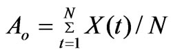
Time series X(t) was represented by decomposition model of additive type
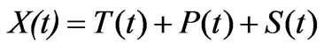
whereT(t)= trend component P(t) = periodic component S(t) = stochastic component
2.6.1. Trend Component
The trend component describes the long smooth movement of variable lasting over the span of the observations, ignoring the short-term fluctuations. The basic idea here is to study only T(t) while eliminating the effects of other components. For detecting the trend, a hypothesis of no trend will be made and following statistical tests, as suggested by [11], were performed:
1) Turning Point Test
2) Kendall’s Rank Correlation Test
2.6.2. Periodic Component
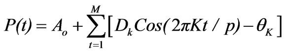
The time series X(t) is expressed in Fourier form as follow:
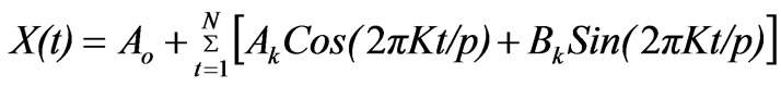 (2)
(2)
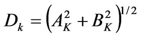
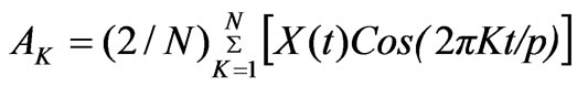
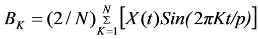
The periodic component concerns an oscillating movement, which is repetitive over a fixed interval of time. Periodic component was determined by the following:
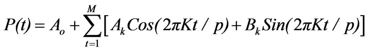 (3)
(3)
It is more convenient to use the alternate form of P(t) given as under:
 (4)
(4)
 (5)
(5)
 (6)
(6)
 =Arctan (
 /
/ )(7)
)(7)
 (8)
(8)
 (9)
(9)
WhereK=number of significant harmonics P=periodicity N=number of observation points Ak and Bk= Fourier coefficientM= number of significant harmonics (maximum, p/2)
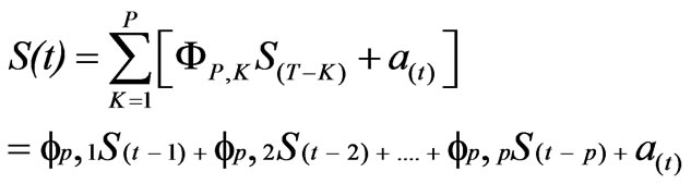
2.6.3. Stochastic Component
The stochastic component is constituted by various random effects, which cannot be estimated exactly. A stochastic model of the form of autoregressive models (AR) will be used for the presentation of the time series. This model was applied to the S(t), which was treated as a random variable and calculated by:
 (10)
(10)
Wherea(t)= independent random number
Φp , K = Autoregressive model parameter =1,2…P
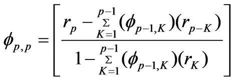
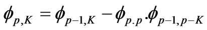
2.6.4. Estimation of the Autoregressive Parameters
These parameters can be expressed in terms of serial correlation coefficient, as Yule–Walker equations. The general recursive formula for estimating these parameters (Φp,K), where suffix p and k indicate the order in AR (p) model, respectively and may be written as:
 (11)
(11)
and
 (12)
(12)
whererK = autocorrelation coefficient For the selection of the order of the AR (p) model residual variance method was used.
2.7. Validation of Stochastic Model
Validation of developed model was performed by comparison of the generated series with the measured historical series. The variation between generated and measured series was presented graphically with respect to time. Linear regression was fitted between generated and measured series.
3. Results and Discussions
The daily black gram evapotranspiration values for twenty-four years (1978-2001) were generated using pan evaporation values. The daily black gram evapotranspiration series was tested for stochastic behavior.
The mean daily series of black gram evapotranspiration has been presented in Figure 1, which confirms the presence of dependent cyclic component and independent part in the series of ETBG.
The findings revels that there is no large variability among the daily values of black gram evapotranspiration of different years. Mean daily values of evapotranspiration ranged 0.8121 to 4.1261mm day-1and standard deviation ranged 0.2217 to 2.0117 mm day-1 during the entire growing season. The variation may be attributed towards the natural change in seasonal climate.
The estimated values of coefficient of variance (CV) of ETBG range from 0.1884 to 0.6888, which signifies the importance of variability ETBG series. Since the values of CV significantly different from zero, it indicates that black gram evapotranspiration is mutually dependent.
The lag one serial correlation coefficient of observed series was found to be 0.686. The values of lag one serial correlation coefficient lie outside the range of confidence limit and are significantly different from zero (Figure 2).This confirms that past and present values of black gram evapotranspiration are highly inter correlated and mutually dependent.
The results of a analysis of coefficient of variance and serial correlation coefficient of different shows that black gram evapotranspiration process is a time variant and not an independent one. Thus, the black gram evapotranspiration time series may be modelled for stochastic process.
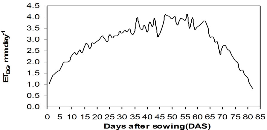
Figure 1. Mean daily black gram evapotranspiration series for 24 years (1978-2001) at Udaipur.
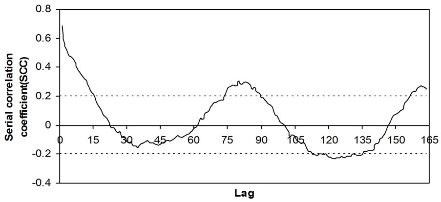
Figure 2. Correlogram of the observed series of black gram evapotranspiration for 24 years (1978-2001) at Udaipur.
3.1. Trend Component
For identification of trend component, annual black gram evapotranspiration series was used [11]. The annual series was obtained by transforming twenty four year seasonal daily evapotranspiration data. For detection, of trend the hypothesis of no trend was made and the values of test statistics (z) was calculated by turning point test and Kendall’s Rank correlation test.
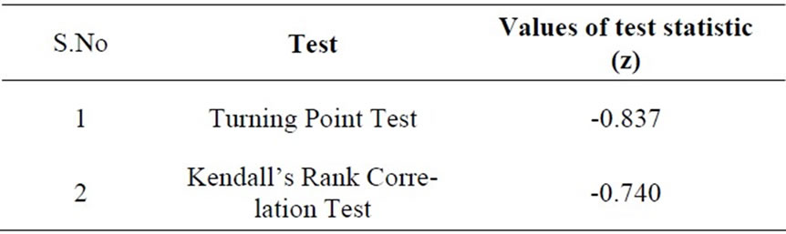
The estimated values of test statistics (zcal) obtained for turning point test, and Kendall’s rank correlation test were within the 1 per cent levels of significance. Hence, the hypothesis of no trend was accepted. So the observed series may be treated as trend free series.
3.2. Periodic Component
The oscillating shape of the correlogram (Figure 2) having peaks at legs equal to 82 and at other multiples of it confirms the presence of periodic component in the daily black gram evapotranspiration series. Therefore, for the harmonic analysis of periodic component, time span of periodicity was taken as 82.
3.2.1. Determination of Significant Harmonics
Numbers of significant harmonics were determined by analyzing the periodic mean daily black gram evapotranspiration series using Equations (8) and (9). Selection of number of significant harmonics performed by conducting F distribution test (Table1) and by plotting cumulative periodogram (Figure 2). The result of analysis of variance indicate that only first three harmonics are highly significant and other harmonics are not significant and, therefore, can be ignored (Table 1).
3.2.2. Parameters of Periodic Component
The first three harmonics explain 92.613 % of the variance. This further confirms that only first three harmonics are significant and may be used to express the periodic component of the daily black gram evapotranspiration series. The values of the Fourier coefficients (A1, A2, A3, B1, B2, B3) were found to be –1.024, -0.42, -0.124, -0.329, 0.057 and 0.018, respectively. Using these six coefficients and Equation (3), the periodic component P(t) from periodic deterministic process may be mathematically expressed as:
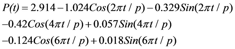 (13)
(13)
The deterministic cycle component P(t) was computed by using Equation (13) for all the values (t=4 to tMAX=1968). A new stationary series S(t) resulting from deterministic stochastic process was obtained, after removing periodic component from the historical series.
3.3. Stochastic Component
The presence of stochastic component was confirmed by plotting the correlogram (Figure 2), periodogram (Figure 3) of observed series, analysis of serial correlation coefficient (SCC) and the coefficient of variance (CV).
The periodic component was removed from the historical series and rest of the series was analyzed to obtain non-deterministic stochastic component by fitting the autoregressive process of stochastic modelling.
3.3.1. Selection of Model Order
Cumulative periodogram was used to determine the order of the model, which may be significantly representing the non-deterministic stationary stochastic component. The maximum variability of Pi 93.8 per cent observed in the first three orders (Figure 3), so order three was select-
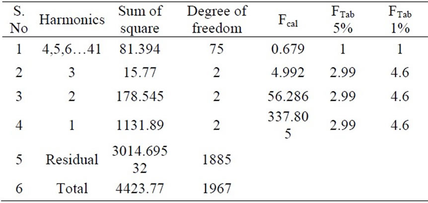
Table 1. Analysis of variance of Fourier coefficient of daily black gram evapotranspiration series of twenty four years (1978-2001).
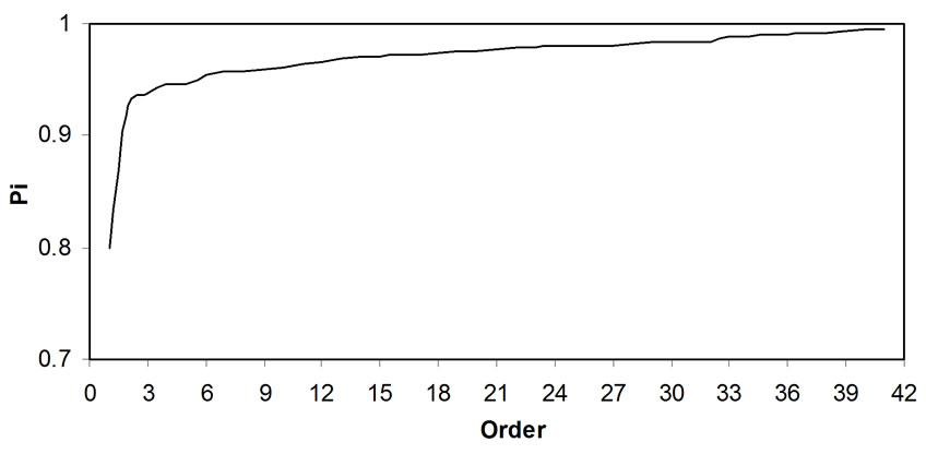
Figure 3. Periodogram of the observed series for black gram evapotranspiration for 24 years (1978- 2001) at Udaipur.
ed to explain the stochastic component of the series.
3.3.2. Mathematical Representation of Stochastic Component
Cumulative periodogram (Figure 2) shows that first three orders explain 92.613 % values while rest explains only 7.38 %. Therefore, autoregressive coefficients (fPP) for first three order were estimated using Equation (11) and (12) as f(3,1)=0.4658, f(3,2)= 0.09552, f(3,3) =0.0933.
The estimated autoregressive coefficient the stochastic component of daily black gram evapotranspiration series may be expressed as:
 (14)
(14)
The non-deterministic stochastic component was estimated by using Equation (14) for all the values (t=4 to 1968).
3.3.3. Residual Series of Stochastic Component
The residual series was obtained after removing the periodic and dependent stochastic parts from the historical series.
The statistical analyses of historical, generated and residual series were presented in Table 2. Residual series shows that the mean is almost equal to zero (0.0003) and standard deviation is equal to one (1.03). The mean, standard deviation and coefficient of variation of the his-
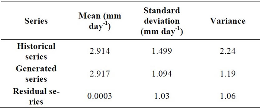
Table 2. Statistical parameters of the historical, generated and residual series of daily black gram evapotranspiration series.
torical and generated series shows closeness between the two.
3.4. Model Structure
Since the observed daily black gram evapotranspiration series was found to be a trend free one, the developed model is a superposition of harmonic deterministic process and third order autoregressive model.
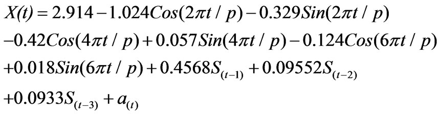 (15)
(15)
3.5. Diagnostic Checking of Black Gram Evapotranspiration Model
The sum of square analysis and analysis of serial correlation coefficient of residual series were performed to test the adequacy of the model. The coefficient of determination (R2) was found to be 0.939, which is nearly equal to unity. This leads to the conclusion that the developed model has a fair goodness of fit to generate the daily black gram evapotranspiration series.
The correlation coefficients for residual series were within the prescribed limits of –0.2 to .20. (Figure 4), which confirm that residual series is purely random series and having neither any periodicity nor any stochastic component. Both tests prove the adequacy of the model.
3.6. Validation of Daily Black Gram Evapotranspiration Series
Validation of generated twenty-four years mean daily black gram evapotranspiration series was made with observed twenty-four years mean daily black gram evapotranspiration series. Figure 5 shows there is linear relationship between ETBGGM and ETBGM series. The correlation coefficient between ETBGGM and ETBGM was found to be 0.96, which is significant at 1 per cent level (Figure 6). The mean values of generated (ETBGGM = 2.9127 mm
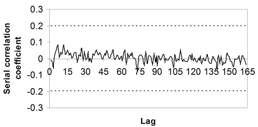
Figure 4. Correlogram for residual series.
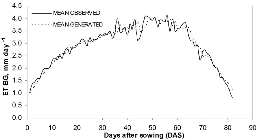
Figure 5. Variation of generated mean black gram evapotranspiration (ETBGM) and observed mean black gram evapotranspiration (ETBGOM).
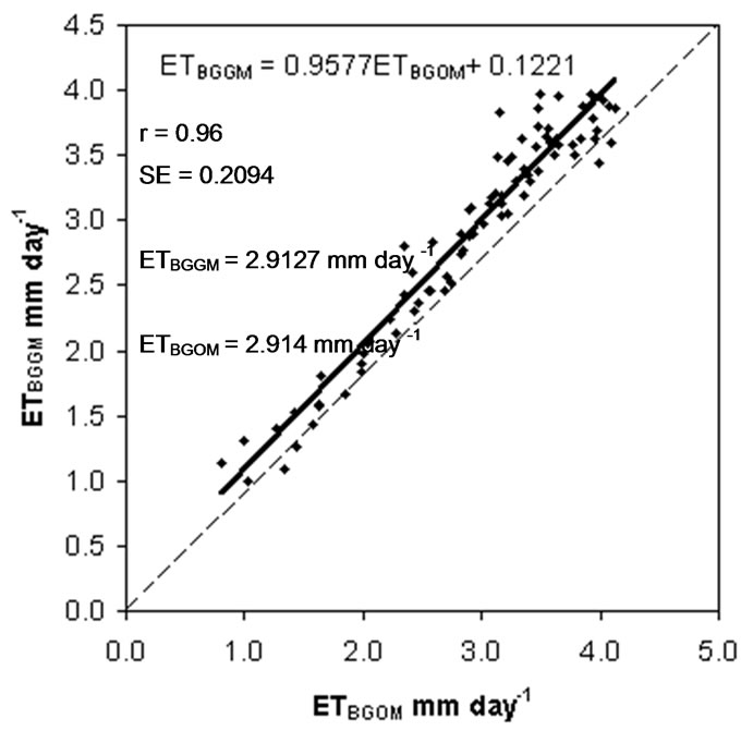
Figure 6. Comparison of generated and observed mean daily black gram evapotranspiration.
day–1) and observed (ETBGM = 2.914 mm day–1) series were very close to each other and standard error (0.2096mm day–1) is quite low. The regression line almost coincide the 1:1 line. Therefore, Equation (15) can be used to predict future values of ETBG quite accurately.
4. Conclusions
The black gram evapotranspiration is time variant and mutually dependent and can be modeled on stochastic theory. It was found that the daily time series of black gram evapotranspiration is trend free and periodic - stochastic in nature with periodicity of 82 days. Hence, the developed model superimposes a periodic deterministic process and a stochastic component results from nondeterministic process. The deterministic periodic component of the average daily black gram evapotranspiration was represented by first three harmonics only. Based on findings it is recommended that the developed model can be used for forecasting black gram evapotranspiration in sub-humid regions and could be applied in similar climatic conditions.
REFERENCES
- J. L. Doob, “Stochastic Processes,” Wiley, New York, 1953.
- P. A. W. Lewis, “Some simple models for continuous variate time series,” Water Resource Bulletin, No. 21, pp. 635–644, 1985.
- J. R. M. Hosking, “Fractional differencing modelling in hydrology,” Water Resources Bulletin, No. 21, pp. 670–682, 1985.
- G. E. P. Box and G. M. Jenkins, “Time Series Analysis, Forecasting and Control,” Holden-Day, San Francisco,
- California, pp 553, 1976.
- J. D. Salas, J. W. Dellur, V. Yevjevich and W. L. Lane, “Applied modelling of hydrologic time series,” Water Resources Publication, Littleton, Coloredo, pp. 484, 1980.
- A. K. Sharma, “Stochastic Modelling for Forecasting Jakham River Inflows,” Ph.D. dissertation, Department of Soil and Water Conservation Engineering, College of Technology and Agricultural Engineering, Rajasthan Agricultural University, Bikaner, pp. 259, 1998.
- R. K. Gupta and R. Kumar, “Stochastic analysis of weekly evaporation values,” Indian Journal of Agricultural Engineering, Vol. 4, No. 34, pp. 140–142, 1994.
- S. R. Bhakar, “Modelling of evaporation and evapotranspiration under climatic conditions of udaipur,” Ph.D dissertation, Faculty of Agricultural Engineering, Department of Soil and Water Conservation Engineering, College of Technology and Engineering, Maharana Pratap University of Agriculture and Technology, Udaipur, 2000.
- D. Kumar, “Modelling of maize evapotranspiration under climatic conditions of Udaipur,” M.Tech dissertation, Faculty of Agricultural Engineering, Department of Soil and Water Conservation Engineering, College of Technology and Engineering, Maharana Pratap University of Agriculture and Technology, Udaipur, 2001.
- R. G. Allen, L. S. Pereira, D. Raes, and M. Smith, “Crop evapotranspiration: guidelines for computing crop requirements,” Irrigation and Drainage Paper, Food and Agriculture Organization (FAO), Rome, Italy, No. 56, pp. 300, 1998.
- N. T. Kottegoda, “Stochastic water resource technology,” The Macmillan Press Pvt. Ltd. London, pp. 384, 1980.
Notation
The following abbreviations and symbols are used in this paper:
Ak,Bk Fourier coefficients at harmonic, K
AR Autoregressive model
CTAE College of Technology and Engineering
ET0 Grass based reference evapotranspiration
ETBG Measured black gram evapotranspiration
ETBGGM Generated evapotranspiration by stochastic model
ETBGOM Observed mean daily black gram evapotranspiration
FAO Food and Agriculture Organization
K Number of significant harmonics
l Lag
M Mean value of stochastic series
p Time span of periodicity
P Order of autoregressive model
Pt Periodic component at time t, t=1, 2,….N
St Stochastic component at time t, t=1,2,….N
Xt Time series of daily black gram evapotranspiration
Yt Trend free series
ak bk Fourier coefficients of periodic mean series of harmonic, k
ФP,K Kth autoregressive coefficient of model order p
ФP,P Partial autoregressive coefficient of model order p
a(t) Independent random number