Journal of Water Resource and Protection
Vol. 1 No. 2 (2009) , Article ID: 617 , 9 pages DOI:10.4236/jwarp.2009.12018
Uncertainty Analysis of Interpolation Methods in Rainfall Spatial Distribution–A Case of Small Catchment in Lyon
1State key laboratory of Pollution Control and Resources Reuse, Tongji University, Shanghai, China
2U.R.G.C. Hydrology Urbane, I.N.S.A. de Lyon, 69621 Villeurbanne Cedex, France
E-mail: taotao@mail.tongji.edu.cn
Received April 7, 2009; revised May 15, 2009; accepted May 18, 2009
Keywords: Rainfall, Spatial Distribution, Kriging, Interpolation
ABSTRACT
Quantification of spatial and temporal patterns of rainfall is an important step toward developing regional water sewage models, the intensity and spatial distribution of rainfall can affect the magnitude and duration of water sewage. However, this input is subject to uncertainty, mainly as a result of the interpolation method and stochastic error due to the random nature of rainfall. In this study, we analyze some rainfall series from 30 rain gauges located in the Great Lyon area, including annual, month, day and intensity of 6mins, aiming at improving the understanding of the major sources of variation and uncertainty in small scale rainfall interpolation in different input series. The main results show the model and the parameter of Kriging should be different for the different rainfall series, even if in the same research area. To the small region with high density of rain gauges (15km2), the Kriging method superiority is not obvious, IDW and the spline interpolation result maybe can be better. The different methods will be suitable for the different research series, and it must be determined by the data series distribution.
1. Introduction
Precipitation is in many cases the most important input factor in hydrological modeling [1]. The role of rainfall is essential for urban hydrology: it is the driving phenomenon of runoff mechanisms, particularly in an urban context. Its variability constitutes a significant source of uncertainty for hydrological modeling. Assessing rainfall variability is an important element to developing conceptual and predictive models of runoff, pollutant loading, and river dynamics. Quantification of spatial and temporal patterns of rainfall is an important step toward developing regional water sewage models. For example, the intensity and spatial distribution of rainfall can affect the magnitude and duration of pollutant washoff to the ocean [2,3], which are also an input for hydrological models. The small size of the urban catchments and the hydrological purposes (especially for real time applications) oblige us to consider rainfall at small scales: on the order of 6 min in time and 5 km in space. Hence urban hydrology requires rainfall measurements with high temporal and spatial resolution.
However, this input is subject to uncertainty, as a result of measurement errors, systematic errors in the interpolation method and stochastic error due to the random nature of rainfall. In addition to the stochastic nature of rainfall, the precipitation pattern may be influenced by the irregular topography. The large variability in altitude, slope and aspect may increase variability by means of processes such as rain shading and strong winds. Accurate estimation of the spatial distribution of rainfall and extrapolation of point measurements over large areas is complicated.
The best method to improve the quality of spatial rainfall estimation is to increase the density of the monitoring network. However, traditionally used rain gauges data are sparse and do not always provide adequate spatial representation of rainfall. This is very costly, and in many cases practically infeasible. And even for dense networks, interpolation remains necessary in order to calculate the total rainfall over a certain area [4]. Therefore, both the design of an adequate monitoring network and choice of an interpolation method require insight in the patterns of rainfall variability and the sources of uncertainty. To provide optimal input for distributed hydrological modeling, the best strategy is probably a combination of all available information on rainfall, including data from hourly point observations, radar data, denser daily measurements, physiographic factors like elevation, and applying sophisticated interpolation or merging methods [5].
Rainfall has been interpolated using averaged values ranging from daily, monthly or annual aggregation levels. And quite a number of modern interpolation methods have been proposed for rainfall. Besides geostatistical approaches, such as ordinary Kriging, Kriging with external drift and co-Kriging [6,7], other techniques based on splines [8,9] or genetic algorithms [10,11] have been applied. These studies concluded that the Kriging method yields a more realistic spatial behaviour of the climatological variable of interest. The use of auxiliary variables in order to improve the spatial interpolation of rainfall variables has been analyzed. Some authors use elevation as an auxiliary variable improving the spatial interpolation of monthly rainfall data, and showing that the interpolation of daily events is improved by the use of elevation as a secondary variable even when these variables show a low correlation [12].
For years various correlation and Semi-Variogram techniques have been used to evaluate both the temporal and spatial structure of rainfall events. Apart from correlation techniques, use of a semi-variogram model for two-dimensional (2-D) interpolation with Kriging approach has been a common practice in different engineering applications, especially in the fields of mining and hydrogeology [13]. By its definition, a semivariogram function has the capability of estimating the disassociation between measurements from the different gauge locations. In hydrologic engineering applications, the semi-variogram development has been applied to estimate the mean precipitation over a catchment by Matheron (1971), Creutin and Obled (1982), Bastin, Larent and Gevers (1984).
In this study, we analyze some rainfall series from 30 rain gauges located in the Great Lyon area (Figure 1), including annual, monthly, daily and intensity of 6mins, which is more useful to water drainage model. Lyon possesses one of the densest rain gauge networks in an urban area within Europe, having 52 gauges in an area of 460 km2. Most of the pluviometers belong to the urban community of Lyon, with 30 tipping bucket rain gauges working in this area. This creates a density of more than 1 pluviometer for every 15 km2. They are spread all over the Lyon area, although with a lower density in the eastern part of the agglomeration. The first rain gauges were set up in 1985, but the actual network density of the present day was reached in 1989. The data is available every 6 minutes although this is variable according to the tip of the bucket.
This paper focuses on three interpolation methods for the different rainfall series. The study is aimed at improving our understanding of the major sources of variation and uncertainty in small scale rainfall interpolation in the time series with different time resolution. This is achieved by means of a spatial characterization and data analysis of the rainfall series. The difference in uncertainty between three interpolation methods that differ strongly in complexity, IDW, Spline and Kriging, is assessed by means of cross validation and validation. This allows us to evaluate the amount of complexity allowed in interpolation, in view of the available data.
2. Methods
Ground-based rain gauge networks supply a reliable source of precipitation data used in many analyses associated with the development of rainfall models. Three methods for the interpolation are used: IDW, Spline and ordinary Kriging. The methods are chosen because they represent two kinds of interpolation methods -- deterministic and geostatistical methods. Each interpolated location is given the value of the closest measurement point, resulting in a typical polygonal pattern and discontinuities at the borders of the polygons. IDW and Spline are deterministic, while Kriging is a geostatistical method. The Inverse Distance Weighted (IDW) and Spline methods are referred to as deterministic interpolation methods because they assign values to locations based on the surrounding measured values and on specified mathematical formulas that determine the smoothness of the resulting surface. Inverse distance weighted (IDW) interpolation determines cell values using a linearly weighted combination of a set of sample points. The weight is a function of inverse distance. The surface being interpolated should be that of a locationally dependent variable. The Spline method is an interpolation method that estimates values using a mathematical function that minimizes overall surface curvature, resulting in a smooth surface that passes exactly through the input points. It fits a mathematical function to a specified number of nearest input points while passing through the sample points. This method is best for generating gently varying surfaces such as elevation, water table heights, or pollution concentrations.
A second family of interpolation methods consists of geostatistical methods, such as Kriging, that are based on statistical models that include autocorrelation (the statistical relationship among the measured points). Because of this, not only do geostatistical techniques have the
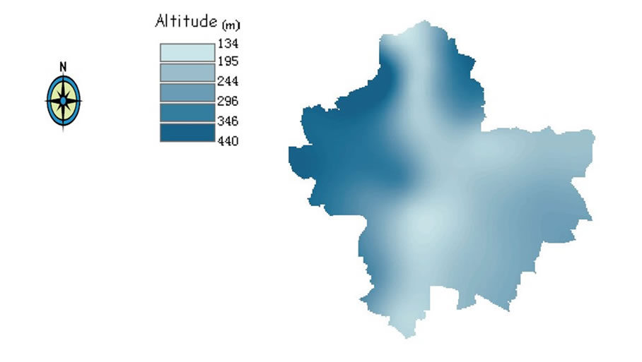
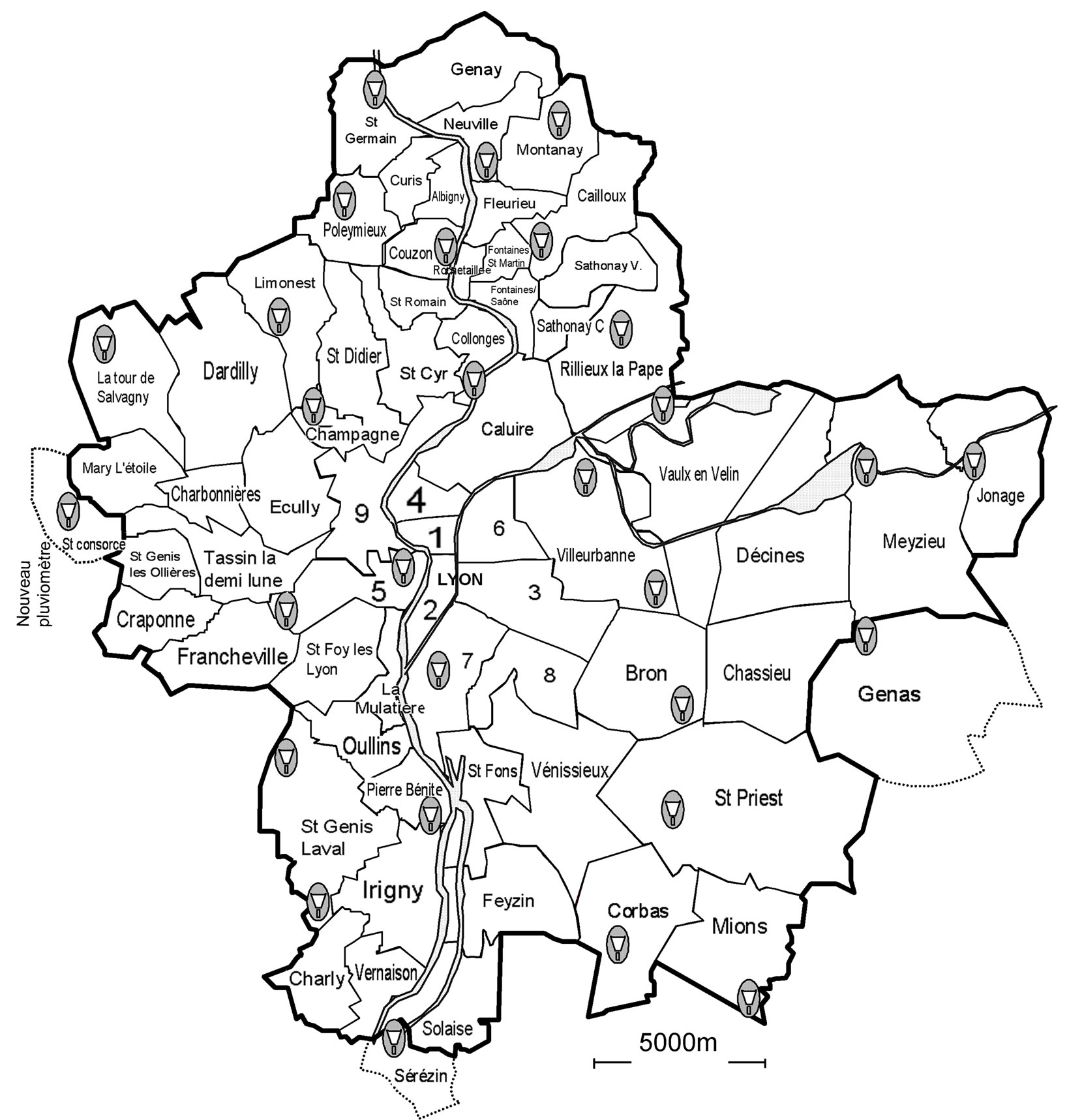
Figure 1. The location of rain gauges in Great Lyon.
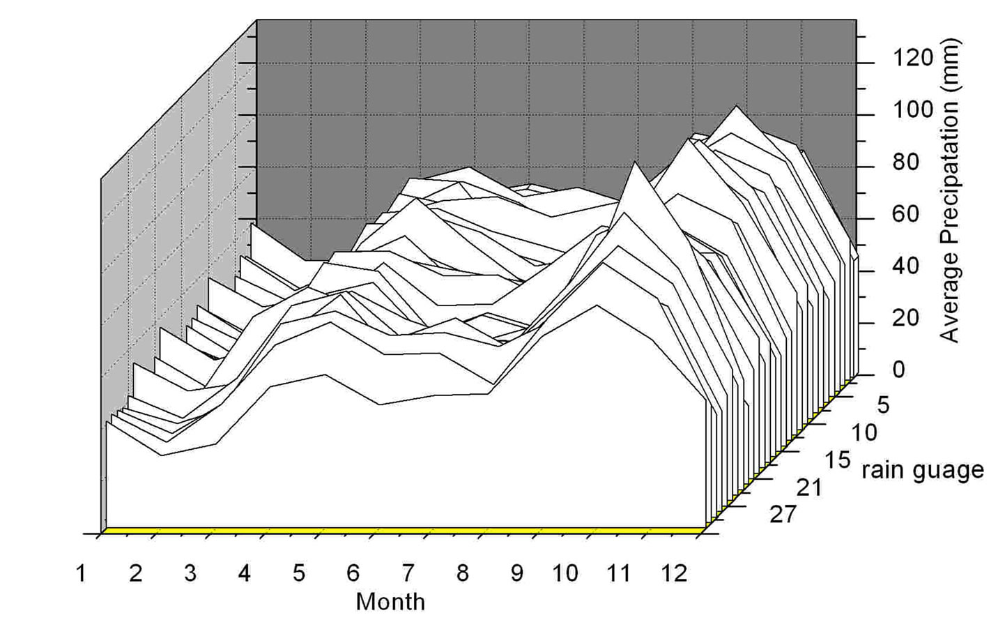
Figure 2. Average monthly precipitation of 30 rain gauges.
capability of producing a prediction surface, but they also provide some measure of the certainty or accuracy of the predictions. Geostatistical Analyst uses sample points taken at different locations in a landscape and creates (interpolates) a continuous surface. The sample points are measurements of some phenomenon such as radiation leaking from a nuclear power plant, an oil spill, or elevation heights. Geostatistical Analyst derives a surface using the values from the measured locations to predict values for each location in the landscape. Kriging is an advanced, computationally intensive, geostatistical estimation method that generates an estimated surface from a scattered set of points with z-values [6,14,15]. Kriging involves an interactive investigation of the spatial behavior of the phenomenon represented by the z-values before the best estimation method is selected for generating the output surface.
Kriging, like most interpolation techniques, is built on the basis that things that are close to one another are more alike than those farther away (quantified here as spatial autocorrelation). The semivariogram is a means to explore this relationship. Pairs that are close in distance should have a smaller difference than those farther away from one another. The extent that this assumption is true can be examined in the semivariogram. Semivariogram measures the strength of statistical correlation as a function of distance.
The semivariogram function is defined as: Y(si, sj) = ½ var(Z(si) - Z(sj)), where var is the variance. si and sj are two locations, Z(si) and Z(sj) are their values.
If two locations are close to each other in terms of the distance measure of d(si, sj), then they are expected to be more similar, so the difference in their values Z(si) - Z(sj), will be small. As si and sj get farther apart, they become less similar, so the difference in their values will become larger. Notice that the variance of the difference increases with distance, so the semivariogram can be thought of as a dissimilarity function.
3. Results and Discussion
The results include three parts: one is to analyze the data, deeper understanding of data will be useful to make decision of model and results analysis; two is to make decision of parameters, such as the choice of semivariogram model, lag size, and search neighborhood, and then according to the cross validation, and comparison of different models, choose the appropriate model for ordinary Kriging interpolation; three is to use the validation to compare the three interpolation methods in annual, monthly, daily and intensity data, and analyze the uncertainty of different methods to different rainfall series.
3.1. Data Analysis
Rainfall data collected from January 1, 1986 to December 31, 2005 on 30 available stations in the whole study area were analized with interpolation technologies. Data with different time span may also have different spatial and temperal distribution. Furthermore, different analysis method should be selected for different data series. In this study, four types of data series were studied, which were annual, monthly, daily, and maxium 6-min precipitation data. Average precipitation in November were selected as monthly rainfall data, because precipitation in this month is always the highest one over 20 years. Precipitation on December 2, 2003 is selected as the oneday rainfall data, because the storm event was happened at this period, and all stations have non-zero rainfall data.
As the distribution of data will affect the selection of methods, we firstly analyzed the Statistical Charateristics of rainfall data. As shown in table 1, the distribution difference of the annual rainfall is not very big, and the Cs (Skewness Coefficient) is only 0.0557. While for the rainfall intensity, the range of variation is bigger and Cs is 0.194, and the biggest Cs is of the rainfall intensity.
3.2. Original Kriging Analysis
This section discusses the impact of different approaches for the estimation of the semivariogram on the original Kriging interpolation performance for different rainfall data series. Because Kriging is a more complicated interpolation process, one special problem for geostatistical interpolation of whole time series is the effective and reliable estimation of the variograms for each time step [5], so special attention is given to the analysis of the impact of the semivariogram estimation on the interpolation performance. First we should have a deeper understanding of the phenomena investigated so that we can make better decisions on issues relating to our data, and then by cross validation and comparing the different models, to choose an appropriate model and parameters.
1) Fit a model—to create a surface and to choose the definition and refinement of an appropriate model.
In the process of Kriging analysis, the semivariogram plays a central role in the analysis of geostatistical data. A valid semivariogram model is selected and the model parameters are estimated before Kriging analysis is performed.
According the history data spatial analysis, notice that the values of the annual rainfall change more slowly in the north–south direction than in east–west the direction. This is because the terrain in east–west direction changes greatly from high to low while the north–south direction
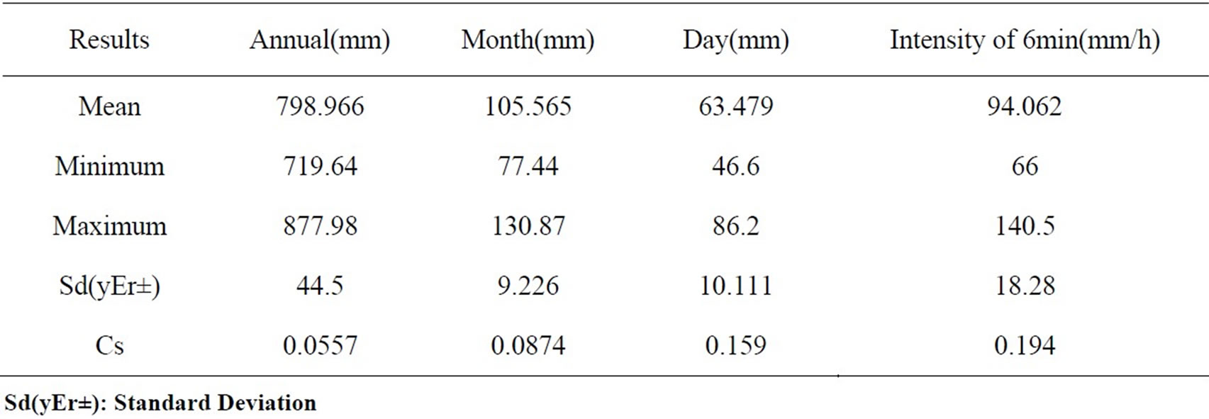
Table 1. of the data series from 30 stations.
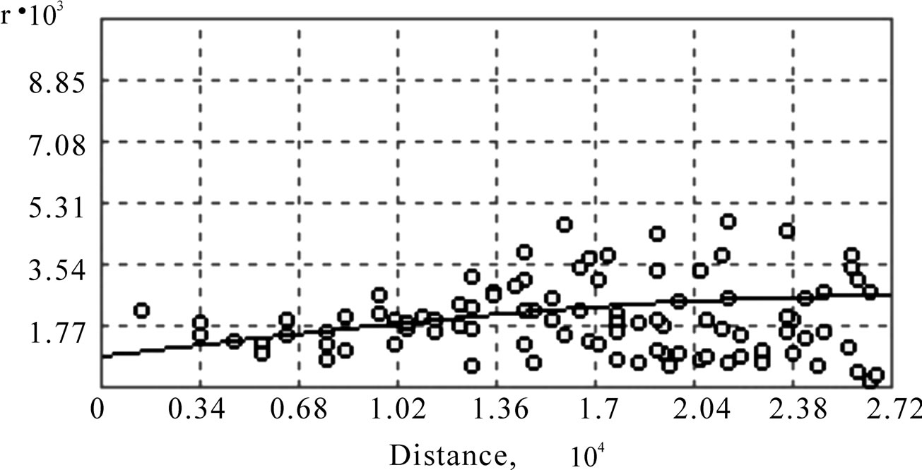
Figure 3. Semivariogram result of annual data.
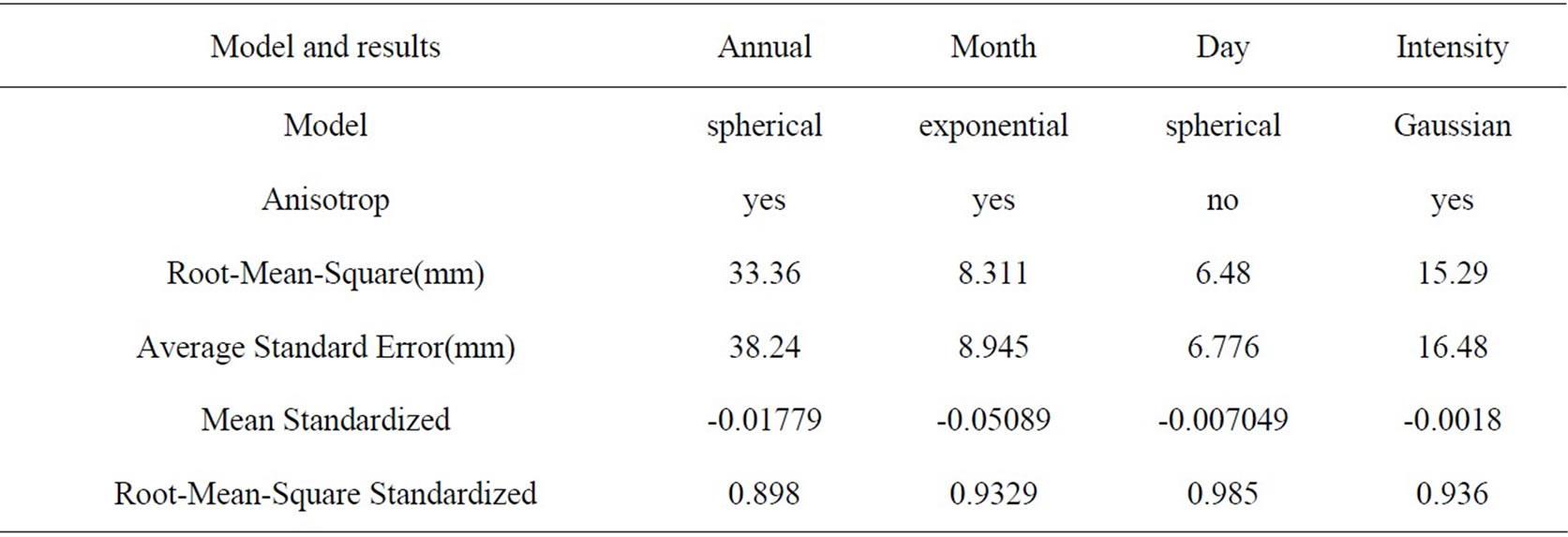
Table 2. Interpolation model parameters and results of different rainfall series.
is more flat. So the anisotropy method is chose. Anisotropy is a characteristic of a random process that shows higher autocorrelation in one direction than another. Annual semivariograms are inferred from annual data considering anisotropic behavior using automatic and manual fitting procedures. Figure 3 shows the semivariogram result of the annual precipitation data, and the parameters of different rainfall series are shown in Table 2.
2) Perform diagnostics—the output surface using cross-validation method, which will help understand how well the model predicts the values at unmeasured locations.
Cross-validation uses the following idea—removes one data locations and then predicts their associated data using the data at the rest of the locations. In this way, we compared the predicted value to the observed value and obtained useful information about some of our previous decisions on the Kriging model. The most rigorous way to assess the quality of an output surface is to compare the predicted values with those measured in the field.
Cross-validation is used to determine "how good" the model is. The goal should be to have standardized mean prediction errors near 0, small root-mean-squared prediction errors, average standard error near root-meansquared prediction errors, and standardized root-meansquared prediction errors near 1.
Table 2 lists the different rainfall series estimation models, parameters and results that are compared here.
Figure 4 shows the standardized error of Kriging interpolation on annual rainfall data. We may conclude from the analysis result that, for the annual rainfalls series from 30 stations, the majority of results of Kriging interpolation is very good with ±5% limits of relative errors. Although the maximum and minimum interpolation errors are a little high, the results are reasonably accepted, because Kriging interpolation is based on the measured value so that the predicted value can not surpass this scope.
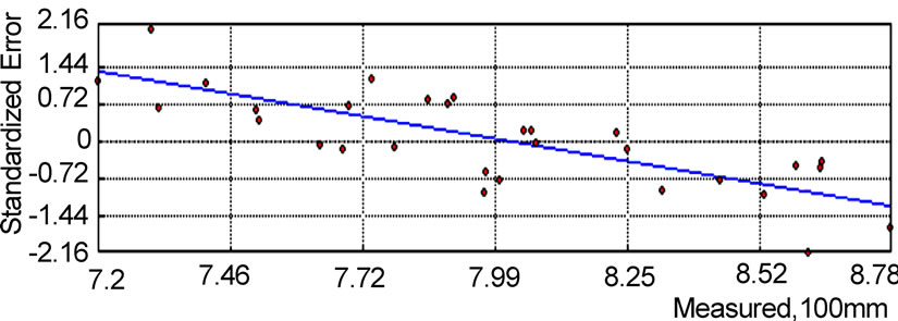
Figure 4. Standardized error of Kriging in annual rainfall.
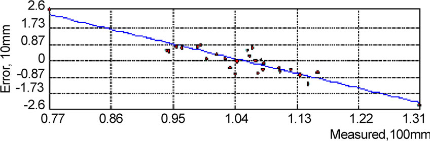
Figure 5. Error of Kriging interpolation in monthly rainfall(mm).
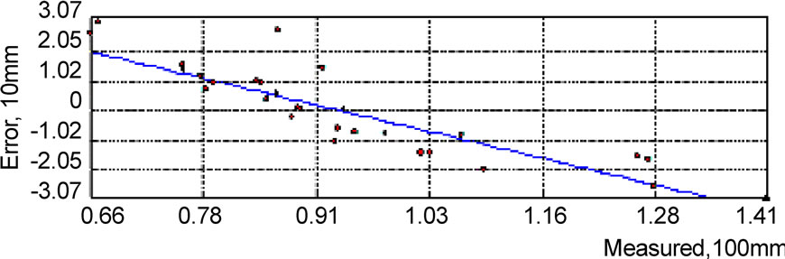
Figure 6. Error of Kriging interpolation in intensity rainfall(mm).
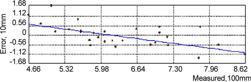
Figure 7. Error of Kriging interpolation in daily rainfall(mm).
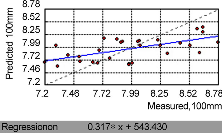
Figure 8. Measured value and predicted value of IDW for annual rainfall.
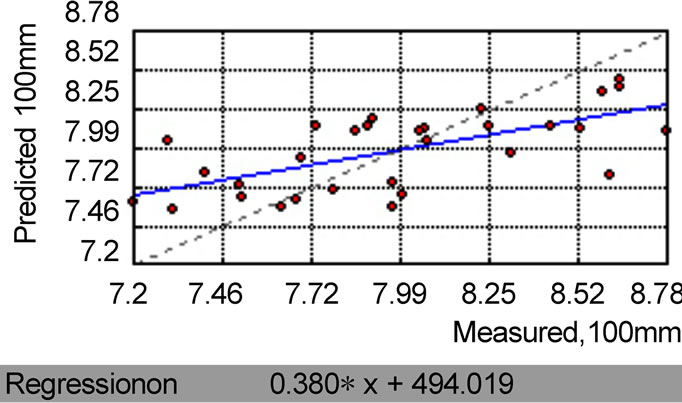
Figure 9. Measured value and predicted value of Kriging for annual rainfall.
The same spatial analysis was carried out in monthly rainfall, daily rainfall and rainfall intensity data, as shown in Figure 5, Figure 6, and Figure 7. The result shows that interpolation on the monthly data series is obviously better than the results on the intensity series and the daily series. The relative errors of monthly series are about within ±8% limits, and we also noticed that the Cs of monthly data serie is obviously smaller than that of the intensity data serie and the daily data seire. Therefore, for the Kriging interpolation method, where there is smaller data variation, there is better interpolation result.
3.3. Results of Three Interpolation Methods
The annual rainfall interpolation results of Kriging and IDW method are shown in Figure 8 and Figure 9. From the regression line of interpolation result, we could see that both methods show good outputs, while the Kriging result (the regression line slope is 0.38) is slightly better than IDW (the regression line slope is 0.317). More detailed analysis results are shown in Table 3-1. For Kriging method, the relative error and std_dev of results are 3.9 and 2.273, while for IDW the values are 2.192 and 3.959. It is believed that the difference of results from these two methods is acceptable. Although neither of these two methods has remarkable advantage in handling with the average annual rainfall data, the spline method will surely get worse results than the above two methods.
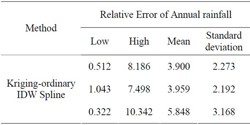
Table 3-1. Validation results of three methods in annual rainfall.
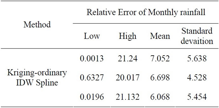
Table 3-2. Validation results of three methods in monthly rainfall.
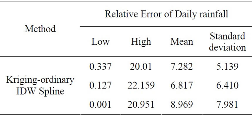
Table 3-3. Validation results of three methods in the daily rainfall.
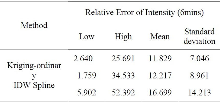
Table 3-4. Validation results of three methods in the intensity (6mins).
For the average monthly rainfall data, result from spline method is comparatively better(shown in Table 3-2), the relative error and std_dev of which are respectively 6.068 and 5.454, while the Kriging result (7.052, 5.638) is inferior to the IDW result. For daily rainfall data, IDW method is the best one (shown in Table 3-3), while spline is obviously worst. For intensity of 6–minute data series, none of the three methods produce high-quality result. Kriging is comparatively good, while the average relative error approaches 11.829 (shown in Table 3-4).
3.4. Uncertainty in Interpolation
These results suggest that most of the uncertainty involved in the interpolation is related to the different basic data statistics. In this view, Kriging is not a better method, as it relies strongly on the assumption of stationarity in the means and thus, a lack of external trends.
In fact, for different rainfall series, it is difficult to determine which method is better. It is not changed with the variation of measured value, its essence should be closely related to the space and temporal distribution of different series. For this study region, because the rainfall station distributed in high density with a small area, the Kriging method cannot show an obvious advantage. At the same time, results from kriging and IDW interpolation are not much different. But for the spline method, the interpolation results in daily rainfall and intensity are not very good. According to statistics analysis of data, we can consider that the spline method is not favorable for data with big Cs .
Although some researchers proposed that in order to reduce the uncertainty of spatial rainfall information, the basic way is to introduce other relative variations with high sample density [6], and to integrate them in interpolation methods. But this suggestion is only suitable for the big area with low distribution density of rain gauges. The choice of those relative variations and their integration with interpolation methods will be one of the main directions of the future research in rainfall interpolation.
4. Conclusions
In this study, different interpolation approaches are compared for the different precipitation series. Special attention is given to the impact of the variogram estimation approach on the interpolation performance. The main results can be summarized as follows:
a) As a kind of geostatistical interpolation methods, the application of the Kriging method obtained the widespread promotion, but in the application process it still had the choice of multi parameters and the model. For the different rainfall series in the same area, its model and the parameter choice of Kriging method may be different.
b) The impact of the semivariogram on interpolation performance is also discussed in this paper. And anisotropy and isotropy are all present in the data, also leading to the little difference in prediction performance. The best results can be obtained using an automatic fitting procedure except isotropic and anisotropic varigrams from all precipitation series.
c) Given the small region with high density of rain gauges (15km2), the Kriging method superiority is not obvious, and to some data series, IDW and the spline interpolation result can be better. Therefore we may obtain, to the different rainfall series, they will be suitable for the different methods, and it must be determined by the data distribution.
In this paper, we have analyzed the connection between data variance and the different interpolation methods, but this kind of data variance that we analyzed is only in the magnitude, not involved spatial distribution. From the characteristic of spatial interpolation, the spatial distribution can be influential to the method selected, so it still needs further to study in this point. Although we concluded that the different data series possibly can be more suitable for different method, the detailed relations between the data and method, at present still has not been able to analyze. Therefore to the small region, if there is no relative information to be applied, selecting the appropriate method will be the key research point.
REFERENCES
- F. Fabry, “Meteorological value of ground target measurements by radar,” Journal of Atmospheric and Oceanic Technology, Vol. 21, pp. 560-573, 2004.
- L. L. Tiefenthaler and K. C. Schiff, “Effects of rainfall intensity and duration on first flush of storm water pollutants,” In S. B. Weisberg, & D. Elmore (Eds.), Southern California Coastal Water Research Project Annual Report 2001-2002, CA’ Westminster, pp. 209-215, 2003.
- J. Vaze and F. H. S. Chiew, “Study of pollutant wash off from small impervious experimental plots,” Water Environment Research, Vol. 39, pp. 1160-1169, 2003.
- P. Goovaerts, “Geostatistics for natural resources evaluation,” Oxford University Press, New York, Oxford, Vol. 483, 1997.
- U. Haberlandt, “Geostatistical interpolation of hourly precipitation from rain gauges and radar for a large-scale extreme rainfall event,” Journal of Hydrology, Vol. 332, pp. 144-157, 2007.
- P. Goovaerts, “Geostatistical approaches for incorporating elevation into the spatial interpolation of rainfall,” Journal of Hydrology, Vol. 228, No. 1–2, pp. 113-129, 2000.
- C. D. Lloyd, “Assessing the effect of integrating elevation data into the estimation of monthly precipitation in Great Britain,” Journal of Hydrology, Vol. 308, No. 1-4, pp. 128, 2005.
- M. F. Hutchinson, “Interpolation of rainfall data with thin plate smoothing splines: Analysis of topographic dependence,” Journal of Geographic Information and Decision Analysis, Vol. 2, No. 2, pp. 152–167, 1998.
- M. F. Hutchinson, “Interpolation of rainfall data with thin plate smoothing splines: Two dimensional smoothing of data with short range correlation,” Journal of Geographic Information and Decision Analysis, Vol. 2, No. 2, pp. 139-151, 1998.
- V. Demyanov, M. Kanevski, S. Chernov, E. Savelieva, and V. Timonin, “Neural network residual Kriging application for climatic data,” Journal of Geographic Information and Decision Analysis, Vol. 2, No. 2, pp. 215-232, 1998.
- Y. Huang, P. Wong, and T. Gedeon, “Spatial interpolation using fuzzy reasoning and genetic algorithms,” Journal of Geographic Information and Decision Analysis, Vol. 2, No. 2, pp. 204-214, 1998.
- J. J. C. Hernandez and S. J. Gaskin, “Spatial temporal analysis of daily precipitation and temperature in the Basin of Mexico,” Journal of Hydrology, doi:10.1016/ j.jhydrol.2006.12.021, 2007.
- K. Umakhanthan and J. E. Ball, “Estimation of rainfall heterogeneity across space and time scale,” Urban Drainage, 2002.
- P. A. Burrough and R. A. McDonnell, “Principles of geographical information systems,” Oxford University Press, 1998.
- C. T. Haan, “Statistical methods in hydrology,” Second Edition, Iowa State Press, 2002.
- G. Bastin, B. Lorent, C. Duque, and M. Gevers, “Optimal estimation of the average area rainfall and optimal selection of raingauge locations,” Water Resource Research, Vol. 20, No. 4, pp. 463-470, 1984.
- J. D. Creutin and C. Obled, “Objective analysis and mapping techniques for rainfall fields: An objective comparison,” Water Resource Research, Vol. 18, No. 2, pp. 251-256, 1982.
- G. F. Lin and L. H. Chen, “A spatial interpolation method based on radial basis function networks incorporating a semivariogram model,” Journal of Hydrology, Vol. 288, 288-298, 2004.
- G. Matheron, “The theory of regionalized variables and its applications,” Ecoledes Mines, Cahiers du Centre de Morphologie Mathematique, Paris, Vol. 5, 1971.
- N. P. Nezlin, E. D. Stein, “Spatial and temporal patterns of remotely-sensed and field-measured rainfall in southern California,” Remote Sensing of Environment, Vol. 96, pp. 228-245, 2005.
- W. Buytaert, R. Celleri, and P. Willems, “Spatial and temporal rainfall variability in mountainous areas: A case study from the south Ecuadorian Andes,” Journal of Hydrology, Vol. 329, pp. 413-421, 2006.
NOTES
*Corresponding author. Foundation item: The Major Science and Technology Project-Water Pollution Control and Treatment (NO.2008ZX7421-001)