Journal of Software Engineering and Applications
Vol. 5 No. 11A (2012) , Article ID: 25191 , 9 pages DOI:10.4236/jsea.2012.531111
Introducing Weighted Nodes to Evaluate the Cloud Computing Topology
![]()
School of Computing, University of Kent, Canterbury, UK.
Email: AAGA2@KENT.AC.UK, frankzgwang@gmail.com, hc269@kent.ac.uk
Received October 14th, 2012; revised November 17th, 2012; accepted November 26th, 2012
Keywords: Adjacency Matrix; Centralities; Geodesic Paths; Weighted Graphs
ABSTRACT
Typical data centers house several powerful ICT (Information and Communication Technology) equipment such as servers, storage devices and network equipment that are high-energy consuming. The nature of these high-energy consuming equipment is mostly accountable for the very large quantities of emissions which are harmful and unfriendly to the environment. The costs associated with energy consumption in data centers increases as the need for more computational resources increases, so also the appalling effect of CO2 (Carbon IV Oxide) emissions on the environment from the constituent ICT facilities-Servers, Cooling systems, Telecommunication systems, Printers, Local Area Network etc. Energy related costs would traditionally account for about 42% (forty-two per cent) of the total costs of running a typical data center. There is a need to have a good balance between optimization of energy budgets in any data center and fulfillment of the Service Level Agreements (SLAs), as this ensures continuity/profitability of business and customer’s satisfaction. A greener computing from what used to be would not only save/sustain the environment but would also optimize energy and by implication saves costs. This paper addresses the challenges of sustainable (or green computing) in the cloud and proffer appropriate, plausible and possible solutions. The idle and uptime of a node and the traffic on its links (edges) has been a concern for the cloud operators because as the strength and weights of the links to the nodes (data centres) increases more energy are also being consumed by and large. It is hereby proposed that the knowledge of centrality can achieve the aim of energy sustainability and efficiency therefore enabling efficient allocation of energy resources to the right path. Mixed-Mean centrality as a new measure of the importance of a node in a graph is introduced, based on the generalized degree centrality. The mixed-mean centrality reflects not only the strengths (weights) and numbers of edges for degree centrality but it combines these features by also applying the closeness centrality measures while it goes further to include the weights of the nodes in the consideration for centrality measures. We illustrate the benefits of this new measure by applying it to cloud computing, which is typically a complex system. Network structure analysis is important in characterizing such complex systems.
1. Introduction
Previously, energy-measurements were carried out manually from the nodes and possibly edges of a network and from the analysis of the data collected predictions can then be made on future-energy consumption. The result from this method deviates greatly from reality and is largely inadequate to give an adequate and reliable prediction of future energy usage. Presently, there are energy-monitoring solutions that collate energy-consumption of the equipment in the data centers, thereby making possible the analysis of data logs, and as such making it easier to predict and identify future trends in energyconsumption.
The above-mentioned task will be more meaningful if the nodes that are idle or low performing are located, and have the weights on their edges re-allocated or re-assigned to the more active nodes that have adequate capacity to accommodate the weights being re-assigned. Moreover, trends in the power consumption behavior of a data center and its nodes could be analyzed in such a manner that future behavior of energy-usage could be predicted with good level of accuracy.
This will go a long way to ensure energy-efficiency and sustainable processes as idle nodes when they are in power-on state still consumes energy and thereby wasting useful and scarce resources.
[1] submitted that “Green” policies should be enforced for energy conservation and sustainable processes (e.g. introducing alerts when power limits are exceeded, thereby indicating which node is consuming or have consumed its fair share of power, the alerts can also trigger automatic adjustments of workload).
Centrality is hereby introduced as a suggested solution to the challenge of allocation of resources or traffic to a node as required. Three basic measures of centrality exists, namely Degree Centrality, Closeness Centrality and Betweenness Centrality, all formalised by [2].
Centrality
Centrality is hereby introduced as a suggested solution to the challenge of allocation of resources or traffic to a node as required. Specifically, a mixed-mean centrality that stems from the idea of Generalizing Degree of Centrality and shortest paths of [3] and Topological Centrality of [4] is hereby proposed. There are three standard measures of centrality namely Degree Centrality, Closeness Centrality and Betweenness Centrality, all formalised by [2]. Each of these centralities either concern itself with nodes or edges [4]. However, this work concerns itself only with the degree and closeness centralities.
2. Standard Centrality Measures
Degree centrality meausre is concerned with the degree of a certain node in a directed graph (or network), that is the number of edges or links or ties that enters a node (wherein referred to as in-degree) or the number of edges that come out of the node (wherein referred to as outdegree), this being applicable to directed graphs. Conversely, in an undirected graph it is the number of ties or edges attached to the node that becomes a concern. Formally, [5] in the Mathematics of Networks defines the degree Ki of a node i is
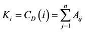 (1)
(1)
where n = number of nodes in the network.
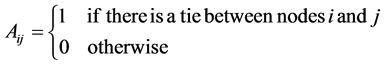 (2)
(2)
by tie, we mean an edge and Aij is an element of the adjacency matrix A, that is, A is an n × n symmetric matrix (implying Aij = Aji). e.g.
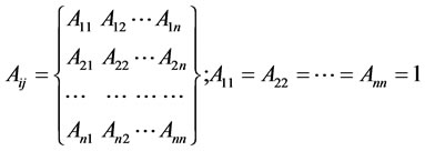 (3)
(3)
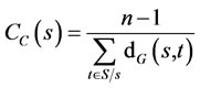
The matrix in (3) above implies that the entry A12 will be equal to A21 if A is an adjacency matrix. The degree centrality has as part of its advantage that only local structure round the node could be known, for ease of calculation this is acceptable, but it becomes a concern if a node is central and not easily accessible to other nodes for one reason or another. It is described by Zhuge [4]
as shown in (4) below:
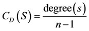 (4)
(4)
where s = node and n = total number of nodes in the graph.
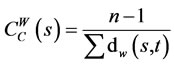
Closeness centrality takes the distance from the focal node to other nodes in a graph into consideration but it has the setback of not taking disconnected nodes (those who are not in the same graph) into consideration. Zhuge [4] formally expresses closeness centrality as
 (5)
(5)
where n = number of nodes, dG(s,t) = geodesic distance between s and t.
Table 1 represents the results of the two standard centrality measures according to Figure 1.
As seen in the table above Node B has the highest of the centralities for the degree and closeness centrality measures.
3. Generalised Degree Centrality Measure
Each of the three standard degrees mentioned above concerns itself with either nodes or edges (Zhuge, [4]). There have been several attempts to generalise the three node centrality measures but most have solely focused on weights of edges and not number of edges (Opsahl et al, [3]). Since weights are of importance, the Equations (4) and (5) above can be extended to include weights, therefore, the weighted degree centrality of node s is hereby represented by
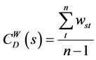 (6)
(6)
where wst is the sum of the weights of edges connected to the particular source node s and, t represents a particular target node. In the same vein, the weighted closeness centrality,  is also represented by
 (7)
(7)
which is the weight of geodesic paths between s and t.
In the attempt to incorporate the measures of both degree and strength of edges (i.e. numbers and weights of edges respectively), [3] considered a graph with 6 nodes (Figure 2) as shown and also introduced the ideal of generalised degree centrality measure.
A tuning parameter α was introduced to take care of the weightedness of the degree and strength of the edges, this being the product of degree of a focal node and the
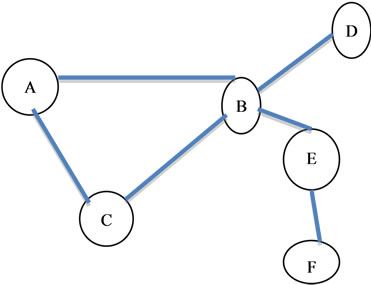
Figure 1. (or Graph 1). A six nodes network, circle represents nodes. (Source: T. Opsahl et al. (2010) p. 245 [3]).
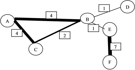
Figure 2. (or Graph 2). A six nodes network, circle represents nodes and square represents weights of edge, e.g. number of visits. (Source: [3], p. 245).
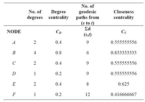
Table 1. Effect of the two basic centrality meausres (degree and closeness centrality measure).
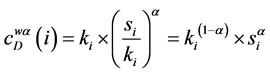
average weight to these nodes as adjusted by the introduced tuning parameter. So, for weighted degree centrality at α we have
 (8)
(8)
where ki = degree of nodes  as defined in (6) above, and α is ≥0.
For weighted closeness centrality at we also have
 (9)
(9)
where ki = degree of nodes while  is as defined in (7) above, where α is ≥0. When applied to Figure 2, Table 2 shows the results for the weighted degree centrality measure and the closeness degree centrality measure.
4. Mixed-Mean Centrality
Introduced hereby is a second similar graph to the one in Figure 2 differing only in the weights attached, it is believed that weights of each tie can actually be dependent on two scenarios (in this case, visit by the focal node and number of messages sent by the nodes through the network). The weights in Figure 2 are the number of visitation by the focal nodes to their neighbors while the weights in Figure 3 below represents the number of messages sent by the focal node, this was applied to a subset of EIES dataset [6].
Figure 3 shows different ranking values for different graphs/or networks, for instance, in Table 3, the first graph (after the application of the tuning parameter to weighted degree centrality measure) made node F to have the highest centrality when , while the same application to the second graph made node A to have the highest centrality. When α < 1, node B has the highest centrality in both cases. Our intention is to combine the results for the two graphs so as to have a fairly well-representative result and not only by using weighted degree centrality but also including weighted closeness centrality.This is reflected in Table 4 .
When the weighted closeness centrality is considered for α > 1, node D has the highest centrality in graph1 while node F has the highest in graph 2, but with α < 1 node B retains the highest centrality position in Graph 1 and in Graph 2.
In Table 5, considering the average (i.e. mean) of the weighted degree centralities for the two graphs; when  returns node A as the most central while with tuning parameter
 , node B is returned as the most central. Whereas the weighted closeness centrality measure when
  and
and  returns node D and node B respectively in both cases as having the highest centrality. From the results above when
 , node B has higher marginal value of cardinality than any other nodes in both graphs.
Table four below presents the results of the MixedMean centralities of the two graphs, that is the summation of the mean of the Weighted Degree and Weighted Closeness centralities. That is,
Mixed-Mean Centralities = (CDW1 + CDW2)/2 + (CCW1 + CCW2)/2 = (CDW1 + CDW2 + CCW1 + CCW2)/2
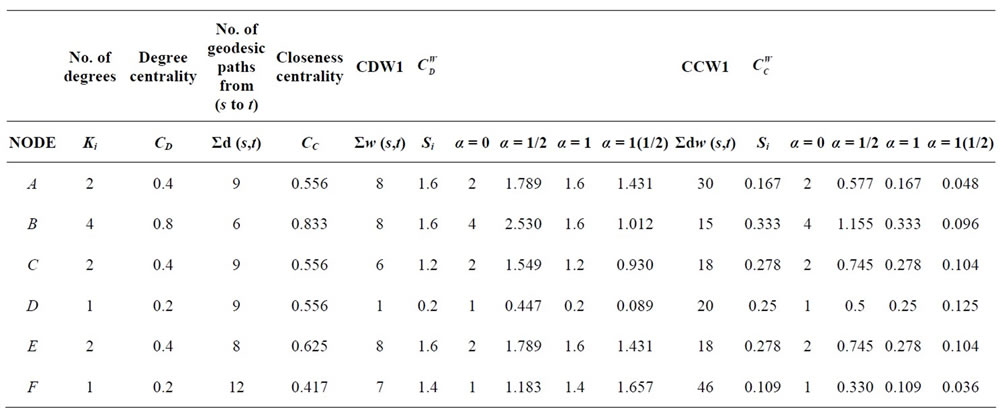
Table 2. Results for the weighted degree centrality measure and the closeness degree centrality measure with the positive tuning parameters.
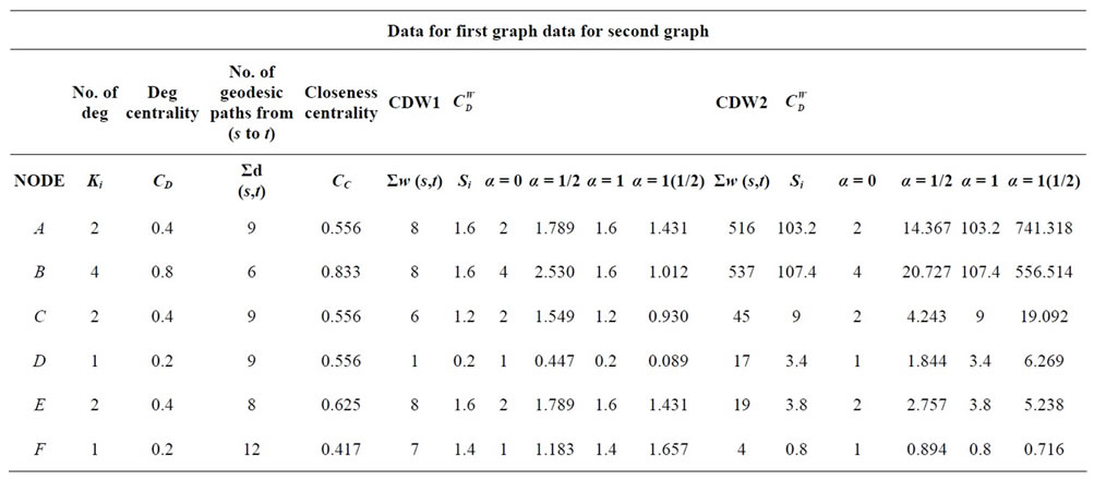
Table 3. Table showing the effect of the tuning parameters on the two graphs of discuss.
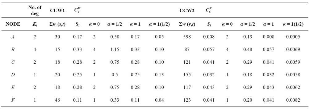
Table 4. The weighted closeness centrality results from the two graphs.
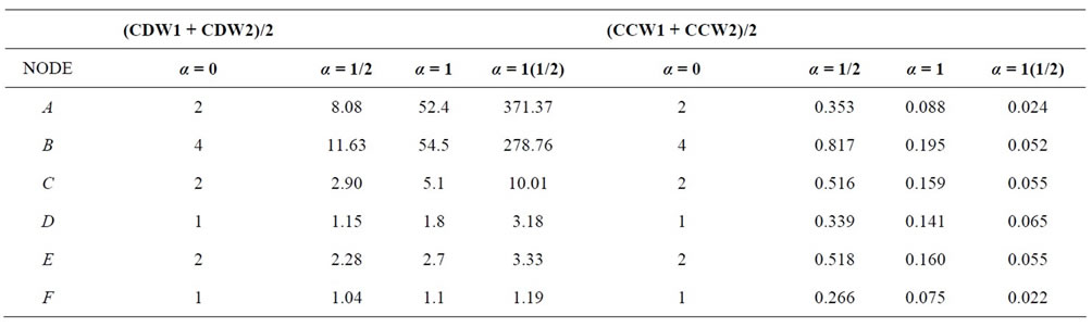
Table 5. The two weighted centralities measure and their averages for the two graphs. (Mean Weighted Centralities for Degree and Closeness Centralities).
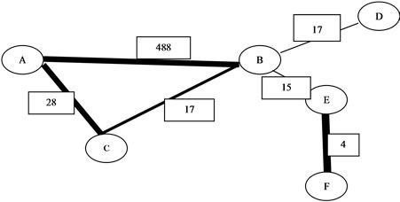
Figure 3. (Graph 3). A six nodes network, circle represents nodes and square represents weights of edge (number of messages).
From the result of Table 6, when  the most central node is B while node A becomes the most central when
 . As shown earlier, in the trivial case when no weights are attached to the nodes (as in Graph1, Table 1), node B is the most central of all nodes as regards degree centrality and closeness centrality. The Table 7 shows the summary result of the activity carried out so far:
In the trivial case of Graph 1, and all other cases whereby the tuning parameter , node B is always the most central. However, the centrality varies when the tuning parameter
 , in fact node B was never the most central in this case, the centrality varies between node D and node F, while for our mixed-mean centrality node A becomes the most central in this case of
 .
.
Application to Data Set
On applying the same to a subset of the Freeman EIES (Electronic Information Exchange System) dataset as presented by Opsahl et al. [3], the Table 8 was generated:
The ranking positions of the mixed-mean weighted centrality above shows the ranking according to the mean of the weightedness of closeness and degree centrality measures at different level of α, thus, it can be inferred that Gary Coombs ranked highest in terms of centralities for both  and
and .
.
However, in terms of the mean of the closeness centralities for both tuning parameters  and
and , it ranked lowest, thereby indicating that the mixture of the centralities for the two graphs could and actually make a less important or influential node to become the most important and influential when considered on the basis of mixed-mean centrality.
5. Mixed-Mean Centrality with Nodes’ Weights
Consideration has been given to weightedness of edges before now, but the nodes can and do have weights, so the principle discussed above is hereby extended to include the node weights for the two graphs of discourse. This means, consideration will now be given not only to the number of ties and tie weights but also to the weights of the nodes. Introducing weights to the nodes of Figure 3, we have the new Figure 4 shown.
Where A (Joel Levine) = 5; B (Jon Sonquist) = 6; C (Brian Foster) = 7; D (Ev Rogers) = 8; E (Gary Coombs) = 9; F (Ed Lauman) = 10 are arbitrary weights assigned to the nodes of the sample EIES data set, these could be the number of resources available to each of the nodes.
The tuning parameter b was now introduced to take care of the weightedness of the nodes, and degree/ strength of the edges, this being the product of degree of a focal node, the average weight to these nodes as adjusted by the introduced tuning parameter and the weight accorded to each node. So, for weighted degree centrality at α and b we shall now have
 (10)
(10)
where ki = degree of nodes  as defined in (7) above zi = weight of nodes, where
 ;
;
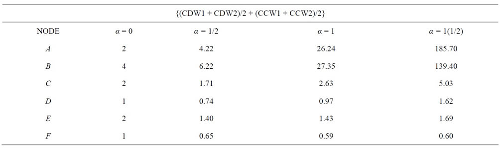
Table 6. Mixed-Mean Centralities of the two Graphs.
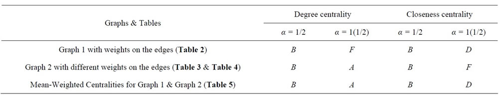
Table 7. A summary of the graphs considered and the most central node in each case.

Table 8. Mixed-Mean Weighted centrality applied to EIES Dataset.
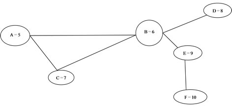
Figure 4. A six nodes network, circle represents nodes and their respective weights using the EIES sample data set.
Applying the new model above to the EIES data set of our discuss will generate the following tables—Tables 9-11 for the new weighted degree centrality (with node weights):
Table 9 shows that when weights are attached to the nodes of the EIES data set, Gary Coombs ranked first while Ed Lauman ranked second when  and
and , whereas in Table 6 whereby the nodes were not accorded weights, Gary Coombs though ranked first but Ed Lauman ranked last, even when the
 .
.
However the above ranking is only for the case whereby the value of , it is quite of interest to us to see what would happen if
 . Table 10 illustrates the result when
 .
.
Table 10 shows that when weights are attached to the nodes of the EIES data set at , Gary Coombs and Joel Levine together ranked first and second respectively when
  but when
  Joel Levine ranked first and Jon Sonquist ranked second.
Finally, the rankings for the different situations of beta after weights z have been attached to the nodes of Table 8 gives the following result:
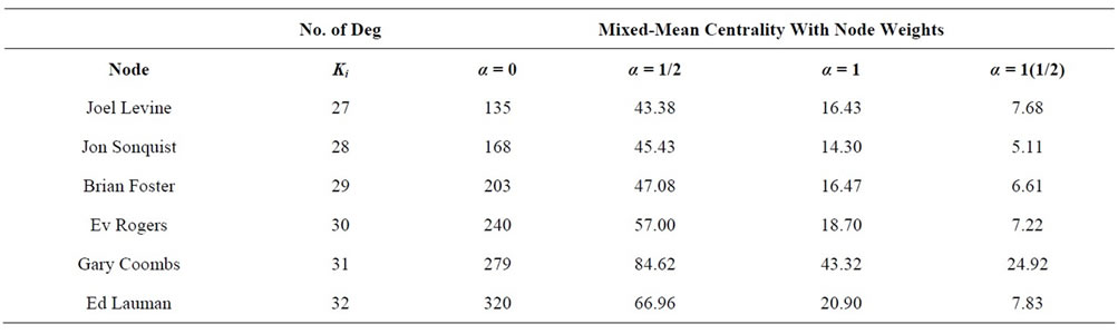
Table 9. Table showing the effect of the tuning parameters on the EIES data sets using the Mixed-Mean Centrality after attaching weights to the nodes, b in this case is 1.
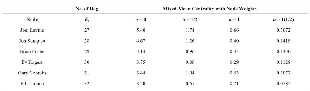
Table 10. Table showing the effect of the tuning parameters on the EIES data sets using the Mixed-Mean Centrality after attaching weights to the nodes, b in this case is –1.
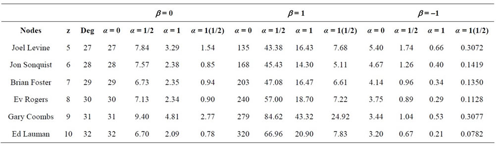
Table 11. Table showing different rankings of nodes after weight z have been attached to the nodes of Table 6 with varying values of b.
From Table 11, it can be seen clearly that as b changes value from 0 to 1 and –1 Gary Coombs (though not the one with highest degree or highest weight) maintains the highest ranking when . When
 , Gary Coombs maintained the lead at
  only to drop to the third position when
 .
.
6. Power Usage Effectiveness (PUE)
It is generally known that even when machines are idle they still consume reasonable energy in that process, but the lower the PUE of a data centre the better and most energy-efficient conscious data centres will always aim to reduce the PUE to the barest minimum, that is conceivably as close as possible to the unit value. As such, one can say that the PUE has a reasonable impact on the energy-efficiency of a data centre.
[7] has this to say about the PUE of its data centres, “In fact, our best site could boast a PUE as low as 1.06 if we used an interpretation commonly used in the industry. However, we’re sticking to a higher standard because we believe it’s better to measure and optimize everything on our site, not just part of it. Therefore, we report a comprehensive PUE of 1.13 across all our data centers, in all seasons, including all sources of overhead.”
An extract of the quarterly PUE from Google’s fourteen (14) data centres spanning the period between 2008 to 2012 is shown in Table 12.
[8] opined that “PUE is defined as the ratio of two numbers, data center input power over IT load power. While it at first appears to be a problem of simply obtaining two measurements and taking their ratio, it rarely is this simple in production data centers”, while Google (2012) postulates the equation below as being a measure of PUE:
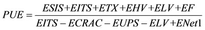 (11)
(11)
ESIS: Energy consumption for supporting infrastructure power substations feeding the cooling plant, lighting, office space, and some network equipment.
EITS: Energy consumption for IT power substations feeding servers, network, storage, and computer room air conditioners (CRACs).
ETX: Medium and high voltage transformer losses.
EHV: High voltage cable losses.
ELV: Low voltage cable losses.
EF: Energy consumption from on-site fuels including natural gas & fuel oils.
ECRAC: CRAC energy consumption.
EUPS: Energy loss at uninterruptible power supplies (UPSes) which feed servers, network, and storage equipment.
ENet1: Network room energy fed from type 1 unit substitution.
Traffic Density Ratio
We introduce a Traffic Density Ratio (TDR) for each of the nodes and it can be described as:
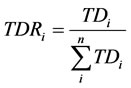 (12)
(12)

Table 12. PUE data for Google’s data Centres.
where TD is the traffic density i = node i and n = total number of nodes in the graph.
The traffic density at each node i is measured in MB/s, and the lower the TDR of a node, the lower the traffic on that particular node, but the TDR is directly proportional to the PUE, that is,
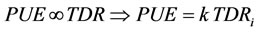 (13)
(13)
where by .
.
Thus, as TDR of any node approaches zero, it is reasonable to believe that the PUE will also tend to zero, and as such all the traffic on such a node could be diverted towards a more performing and capable node, while the node whose PUE is almost at zero could be shut down, thereby saving much energy.
7. Future Studies
1) The concept developed herein shall be applied to real data from cloud data centres.
2) The tuning parameters α and b can each be considered as a range of values, thereby introducing dynamism as a measure of centrality.
3) While considering the centrality for the location of the high/low energy consuming nodes/edges, other important factors to take into cognizance are the Power Usage Effectiveness (PUE) and Traffic Density Ratio (TDR).
8. Contribution
1) Two graphs were considered and effects of the combined weights on both edges and nodes were evaluated taking the closeness centrality and degree centrality into cognisance.
2) The resulting Mixed-Mean centrality was then applied to the EIES data set while introducing two tuning parameters α and b.
9. Conclusions
The scenario presented here can be applied to cloud computing by using the idea of mixed-mean centrality to discover the most central and therefore the most energy consuming nodes, so as to help in making provision for energy-efficiency, thus minimising costs and saving the environment. It can be used in locating the performance level of a particular node or edge and thus aiding in decision on which node or edge deserves attention. This can be most especially useful for security and faulttolerance purposes.
Resource allocation is also an applicable area of this centrality measure as it will aid in optimisation of resources, thereby saving costs.
10. Acknowledgements
The contribution of Dr. Matteo Migliavacca is hereby acknowledged for his constructive criticsm during the course of this work.
REFERENCES
- S. Klaus, “Data Center Energy: Past, Present and Future,” 30 September 2012. http://www.datacenterjournal.com/it/data-center-energy-past-present-and-future-part-one/?goback=%2Eanb_61513_*2_*1_*1_*1_*1_*1
- L. C. Freeman, “Centrality in Social Networks: Conceptual Clarification,” Social Networks, Vol. 1, 2012, pp. 215-239. http://moreno.ss.uci.edu/27.pdf
- T. Opsahl, F. Agneessens and J. Skvoretz, “Node Centrality in Weighted Networks: Generalizing Degree Shortest Paths,” Social Networks, Vol. 32, 2010, pp. 245-251. doi:10.1016/j.socnet.2010.03.006
- H. Zhuge and J. Zhang, “Topological Centrality and It’s e-Science Applications,” Wiley Interscience, New York, 2010.
- M. E. J. Newman, “The Mathematics of Networks,” Center for the Study of Complex Systems, University of michigan, Ann Arbor, 6 June 2012. http://www.personal.umich.edu/~mejn/papers/palgrave.pdf
- S. C. Freeman and L. C. Freeman, “The Networkers Network: A Study of the Impact of a New Communications Medium on Sociometric Structure,” Social Science Research Reports S46, University of California, Irvine, 1979.
- Google, “Efficiency How We Do It,” 1 October 2012. http://www.google.com/about/datacenters/efficiency/internal/index.html#measuring-efficiency
- V. Avela, “Guidance for Calculation of Efficiency (PUE) in Data Centres. White Paper 158,” Schneider Electric’s Data Centre Science, 2011.