iBusiness
Vol.2 No.1(2010), Article ID:1444,10 pages DOI:10.4236/ib.2010.21009
Influence of Lateral Transshipment Policy on Supply Chain Performance: A Stochastic Demand Case
![]()
1School of Business, Nantong University, Nantong, China; 2Institute of Logistics Engineering, Nantong University, Nantong, China.
Email: carl.jxchen@hotmail.com, jxchen@ntu.edu.cn
Received September 14th, 2009; revised October 25th, 2009; accepted December 2nd, 2009.
Keywords: Supply Chain, Inventory System, Lateral Transshipment, Performance
ABSTRACT
Considering the supply chain consists of one supplier and two retailers, we construct the system’s dynamic models which face stochastic demand in the case of non-lateral transshipment (NLT), unidirectional lateral transshipment (ULT) and bidirectional lateral transshipment (BLT). Numerical example simulation experiments of these models were run on Venple. We adopt customer demand satisfaction rate and total inventory as performance indicators of supply chain. Through the comparative of the simulation results with the NLT policy, we analyze the influence of ULT policy and BLT policy on system performance. It shows that, if retailers face the same random distribution demand, lateral transshipment policy can effectively improve the performance of supply chain system; if the retailers face different random distribution demand, lateral transshipment policy cannot effectively improve the performance of supply chain systems, even reduce system’s customer demand satisfaction rate, and increase system inventory variation.
1. Introduction
Lateral transshipment, an important inventory replenishment policy, has gained a common concern of the academics and business managers in recent years. There are numerous researches about this issue. Lateral transshipment is defined as the redistribution of stock from retailers with stock on hand to retailers that cannot meet customer demands or to retailers that expect significant losses due to high risk [1]. The early pioneering work of Krishnan and Rao [2] examine a periodic review policy in a single-echelon, single-periodic setting [2]. Robinson [3] extends the research to a multi-period case, and establishes the system’s lateral transshipment model [3]. The emergency lateral transshipment model of repairable product was analyzed by Lee [4] for the two-echelon inventory system case [4]. Axsäter [5] studies the emergency lateral transshipment problem of the multi-level repairable product inventory system, and gets some interesting conclusions different from Lee’s [5]. Archibald et al. [6] develop a lateral transshipment model among the multi-retailer based on Markov decision-making methods [6]. Grahovac and Chakravarty [7] limit the research object to low demanded expensive product and analyze the lateral transshipments model in a multiechelon supply chain system [7]. Kukreja et al. [8] consider a single-echelon continuous review inventory system which contains n depots, and takes the expensive consumable product as object, study the one-to-one lateral transshipment model [8]. Rudi et al. [9] work on optimal order policy of the vendors in the existence of lateral transshipment circumstances [9]. Minner and Silver [10] provide a new decision rule of system’s lateral transshipment, and prove it can figure out the size of transshipment as well as some important problems [10]. Xu et al. [11] analyze emergency lateral transshipment policy between the two-echelon continuous review inventory system that use  policy [11]. Banerjee et al. [12] study lateral transshipment of two-echelon supply chain systems which include multiple retailers and single supplier based on DOE [12]. Xu and Luo [13] use Expect Cost Method to analyze lateral transshipment policy in cross-docking system [13]. Xu and Xiong [14] analyze the best time for one-off transshipments in a cross-docking system with stochastic demand [14]. Wang et al. [15] conduct a quantitative analysis to the value of lateral transshipment policy of regional inventory distribution systems, which consist of a distribution center and multiple retail points [15]. Huo and Li [16] develop batch ordering policy in a single-echelon, multi-location transshipment inventory system [16]. Li et al. [17] study inventory management model of the cluster supply chain system with the existence of emergency lateral transshipment [17].
Most of the papers above dealing with transshipment assume that lateral transshipment already exists in system. However, lateral transshipment will make the problem complicate and tend to be very difficult to analyze analytically, especially BLT [18]. Hence, will lateral transshipment really need? This paper handles this problem from the performance measurement point. We consider one supply chain system consists of one supplier and two retailers, allowing a retailer transship from the other one for inventory replenishment besides order from supplier. System’s models were developed by system dynamics assume that all the members use the order-up-to policy, and numerical experiment was run on Venple platform.
The paper is organized as follows: in Section 2, the models with lateral transshipment were developed, as well as without lateral transshipment. The accuracy of the model is tested against simulation in Section 3; Section 4 deals with the influence of ULT and BLT. The conclusion of this paper was presented in Section 5.
2. Model Description
We consider two retailers facing independent stochastic customer demand and one supplier (Figure 1). Without lateral transshipment, retailers order from suppliers to replenish inventory in case of stock out. In order to respond to customer demand quickly, they can use lateral transshipment policy besides order from the supplier, which means they replenish inventory from the other one if there exist surplus stock on hand.
2.1 Model Assumption
Development of the model needs the following assumptions.
• Customer1 and Customer2 face independent stochastic demand;
• Both retailers adopt order-up-to policy, the ordering period is constant;
• Lateral transshipments take no time;
• Transshipments take place when there are surplus stocks. That is, if retailer 1 needs transshipment from retailer 2, retailer 2 only transships the redundant stock.
2.2 System Model
As a modeling and simulation technology, system dynamics has a wide range of applications since its birth, especially in dealing with long-term, chronic, dynamic management problems [19]. Forrester [20] applies system dynamics in industrial business management, addressing issues such as fluctuations in production and employees, instability of market shares and market growth [20]. Logistics and Supply Chain Management is an important area of System Dynamics. Sterman [21]designs the well-known beer game by System Dynamics, and carries out detailed analysis on feedback loops, nonlinear, time-delay and management behavior in the system [21]. Diseny et al. [22] analyze VMI in transport operation by system dynamics [22]. Marquez [23] establishes a model for measuring financial and operational performance in the supply chain based on System Dynamics [23], and so on.
Generally speaking, a complete system dynamics model usually consists of three parts: model variables, causal loop diagrams and mathematical description. We analyze the three part of model in turn as follows.
2.2.1 Model Variables
The structure of a system dynamics model contains stock, smoothed stock, flow rate, auxiliary variables and constants. Stock variables are used to describe the cumulative effect of the system. Smoothed stock variables are the expected values of specific variables obtained by exponential smoothing techniques. Flow rate describes the rate of the cumulative effect of the system. Auxiliary variables are the middle variables which express the decision-making process. Constants change little or relatively do not change during the study period. The fundamental notations of the model are following:

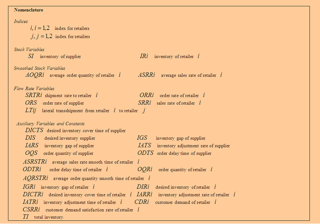
Figure 1. 2-echelon supply chain. Filled arrows represent the flow of regular replenishments while dashed arrows represent the lateral transshipment flow
2.2.2 Causal Loop Diagrams
Causal loop diagram is a tool that expresses the structure of the system, playing an extremely important role in system dynamics. There are two reasons for that. First, during model development, they serve as preliminary sketches of causal hypotheses and secondly, they can simplify the representation of a model.
The first step of our analysis is to capture the relationship among the system operations in a system dynamics manner and to construct the appropriate causal loop diagram.

Figure 2. Causal loop diagram of the supply chain without lateral transshipment
Figure 2 describes the causal loop of the supply chain without lateral transshipment.
The system structure in Figure 2 contains supplier and retailers. For the supplier,  is decided by
  and
and .
.  is determined commonly by
  and
and . Delivery rate
  is determined by
  and
and . Supplier adjust inventory level by setting
 , together with
  determine
 .
.  and
and  determine
 , in turn,
  has a direct impact on
 and an indirect impact on
 . For retailers,
  is determined by
  and
and .
.  is the delay of
 , delay time is
 .
.  is decided by
  and
and .
.  is obtained from
  after the time
 . Retailers also adjust inventory level by setting
 .
.  is decided by
  and
and .
.  and
and  jointly determine
 .
.  and
and  commonly determine
 . If
. If  is greater than 0, Retailer sent orders to suppliers, order quantity
  is decided by
 .
. ,
,  , and
, and  determine
 . There are two performance variables, customer demand satisfaction rate
  and total inventory
 .
.  is decided by inventory
  and customer demands
 ,
,  is a accumulation sum of supplier inventory
  and
and .
.

Figure 3. Causal loop diagram of the supply chain with unidirectional lateral transshipment
Figure 3 describes the causal loop diagram of supply chain with ULT.  means the transshipment from retailer 2 to retailer 1. It is a flow rate variable and means that when retailer 1 out of stock, retailer 2 will replenish retailer 1 by transshipment on condition that it has surplus stock.
  is decided by
  and
and , and influence
 .
.

Figure 4. Causal loop diagram of the supply chain with bidirectional lateral transshipment
Figure 4 describes the causal loop diagram of the supply chain with BLT.  is the same as noted above.
 ![]() is a flow rate variable and means that when retailer 2 is out of stock, retailer 1 will replenish retailer 2 by transshipment on condition that it has surplus stock.
is a flow rate variable and means that when retailer 2 is out of stock, retailer 1 will replenish retailer 2 by transshipment on condition that it has surplus stock.
![]() is decided by
is decided by  and
and , and influence
 .
.
2.2.3 Mathematical Description
The next step of system dynamics methodology includes the development of the mathematical model, usually presented as a stock-flow diagram that captures the model structure and the interrelationships among the variables. Combining mathematical description and causal loop diagram of variables, we use visual simulation software (Venple) to reflect the behavior of the system and provide a basis for decision-making. We analyze the mathematical description of the main variables in the system under the three cases of NLT, ULT and BLT so as to lay a good foundation for model simulation.
NLT case
 (1)
(1)
 (2)
(2)
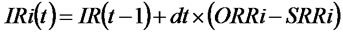
(1) is the inventory dynamics equation of supplier, (2) is the inventory dynamics equation of retailer .
.
 (3)
(3)
 (4)
(4)
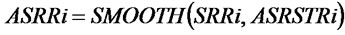
(3) is the average order quantity equation of retailer , (4) is the average sales rate equation of retailer
 .
.
 (5)
(5)
 (6)
(6)
 (7)
(7)
 (8)
(8)
(5) and (6) are the order rate equations of suppliers and retailers, which are the delay function of the corresponding order quantities in a given period of time. (7) is the equation of supplier shipment rate to retailers. It means when ,
,  is 0; when
  and the total order quantity
![]() , supplier can fully meet the orders of retailers, shipment rate is the order quantity of retailers
, supplier can fully meet the orders of retailers, shipment rate is the order quantity of retailers ; when
  and
and , supplier partly meet the orders of retailers. According to the proportion of orders, shipment rate is
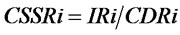
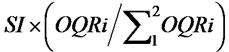 . (8) is the sales rate equation of retailer
 . When
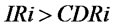 , meaning that customers’ demand will be met completely,
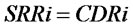 ; When
 , meaning that the customer demand will be met partly,
 ; when
 , meaning that the customer demand will never be met,
 .
.
 (9)
(9)
 (10)
(10)
 (11)
(11)
 (12)
(12)
 (13)
(13)
 (14)
(14)
 (15)
(15)
 (16)
(16)
 ,
, ,
, ,
, ,
, ,
, ,
, and
and are constant.
(9)~(13) are the auxiliary variables equations of supplier. (9) is the desired inventory equation of supplier. (10) is the order rate equation of supplier. (11) is the inventory gap equation of supplier. (12) is the inventory adjustment rate equation of supplier. (13) is the ordquan tity equation of supplier. When  or
or
 ,
, ; When
  and
and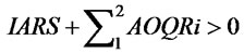 ,
,![]() . (14)~(16) express the auxiliary variables equations of retailers. (14) and (15) express the desired inventory equation and the inventory gap equation of retailer
. (14)~(16) express the auxiliary variables equations of retailers. (14) and (15) express the desired inventory equation and the inventory gap equation of retailer . (16) is the order quantity equation of retailer
 . When
  or
or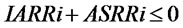 ,
, ; When
  and
and ,
, .
.
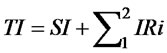 (17)
(17)
 (18)
(18)
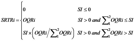
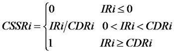
(17) is the total inventory equation of the supply chain system. (18) is the customer demand satisfaction rate equation of the supply chain system. When ,
, ; When
 ,
, ; When
 ,
, .
.  is a random variable, and it obeys a certain random distribution.
ULT case.
 (19)
(19)
 (20)
(20)
 (21)
(21)
 (22)
(22)
 (23)
(23)
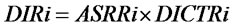
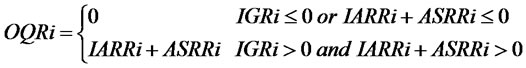
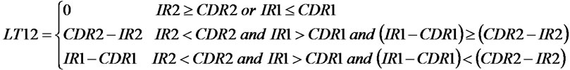
(19)~(23) are the equations of variables in the ULT situation, and the other variables which were not include in the above expression are the same as the variables in the NLT situation. (19) is the transshipment rate equation. When  or
or ,
, ; When
 ,
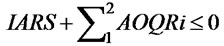
,  and’
and’ ,
, ;
;
 ,
, ;
;
When ,
,  and
and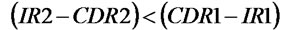 ,
,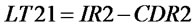 . (20)~(23) express the variables changed in ULT, and their explanations are similar with NLT.
BLT case.
 (24)
(24)
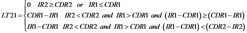 (25)
(25)
 (26)
(26)
 (27)
(27)
 (28)
(28)
 (29)
(29)
(24)~(29) are the equations of variables in the BLT situation, and the other variables which were not included in the above expression are the same as the variables in the NLT. The explanations of above equations are the same as the ULT case, and the concrete explanations will be omitted.
3. Models Validation
The main criterion for system dynamics models validation is structure validity, which is the validity of the set of relation used in the model, as compared with the real process. For detection of structural flaws in system dynamics models, certain procedures and tests are used. These structure validity tests are grouped as direct structure tests and indirect structure tests. Direct structure tests involve comparative evaluation of each model equation against its counterpart in the real system (or in the relevant literature). Direct structure testing is important, yet it evolves a very qualitative, subjective process that needs comparing the forms of equations against real relationship. It is therefore, very hard to communicate to others in a quantitative and structured way. Indirect structure testing, on the other hand, is a more quantitative and structured method of testing the validity of the model structure. The two most significant and practical indirect structure tests are extreme-condition and behavior sensitivity tests [24]. Generally, the goal of extreme test lies in whether the equations are still meaningful or not and whether the model conditions are still reasonable or not under the situation of using extreme input. Behavior sensitivity test consists of determining those parameters to which the model is highly sensitive and asking if these sensitivities would make sense in the real system. If we discover certain parameters to which the model behavior is surprisingly sensitive, it may indicate a flaw in the model equations.
In view of the deficient of real data and the difficulty of gaining mass data, we only use the extreme condition test and the sensitive test in the indirect structure tests to carry on the validation for the models of this paper. We use the total inventory which is a main output of the system to confirm the performance in the extreme test and the sensitive test.
Suppose that the system is facing an extreme demand, we use Venple to test the models which are NLT, ULT and BLT, and compare the simulation results with the normal demand case. The results are shown in Figure 5. Although the total inventory becomes very big with the sharply increasing demand, the tendency is similar with the normal demand case. This indicates that the variables and the equations in the system still have effects, and the model displays a good robustness under the extreme input.
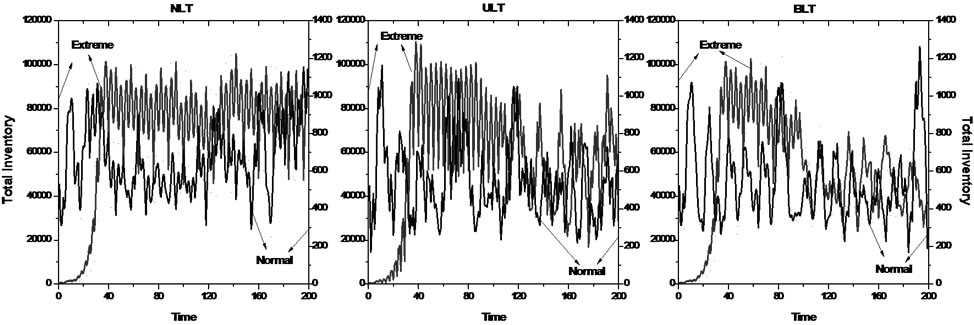
Figure 5. Total inventory in normal condition and extreme condition
Through changing the demand parameters, we use Poisson distribution to test the models’ sensitivity, and the simulation experiment is also carried on the Venple.
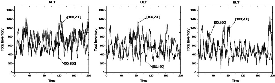
Figure 6. Total inventory of two different kinds of demand
Figure 6 presents the result that compare with the normal parameters case. We can see although fluctuation range of the total inventory is inconsistent under the two kinds of demand with different parameters, the tendency displays as basically consistent. This explains that the models don’t sensitively response to the parameters, and this is conducive for the model’s practical application.
4. Numerical Simulation
We employ a numerical example to examine the influence of three different policies on system performance, and further analyze the simulation results and provide reasonable suggestions. In order to facilitate the numerical simulation, we set the initial value of the constants,  ,
,  ,
,  ,
,  ,
,  ,
,  ,
,  ,
,  ,
,  ,
, . Where
 ![]() is the simulation time.
is the simulation time.
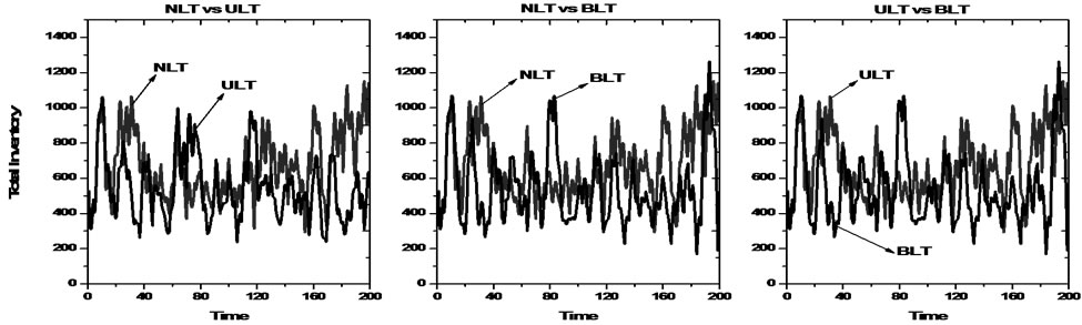
Figure 7. Total inventory in the same distribution demand case
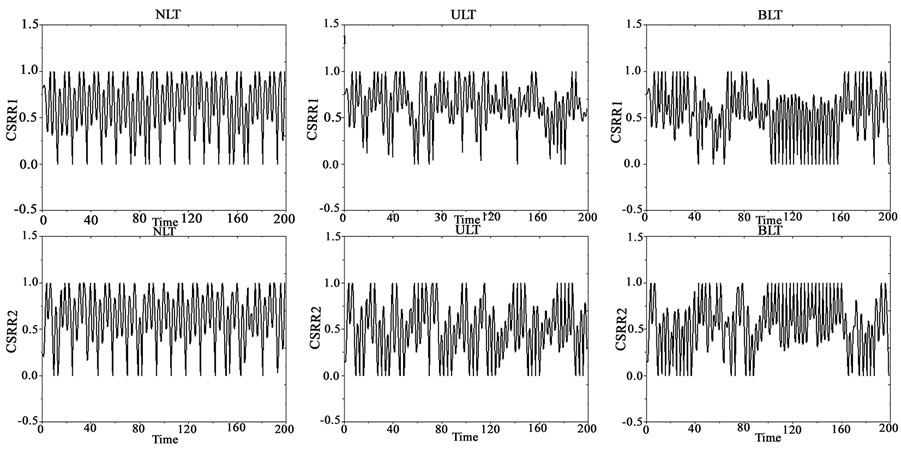
Figure 8. Customer satisfaction rate in the same distribution demand case
4.1 Same Distribution Demand Case
We assume retailer i face same distribution demand that is Poisson distribution with range from 50 units to 150 units. Simulation results are shown in Figure 7, Figure 8 and Table 1.
From the simulation results, the system has the lowest total inventory in BLT case, the average size is 540.2057 units and the standard deviation is 192.2115 units; The following is that in ULT case with its mean is 546.1087 units and the standard deviation is 199.2071 units; Under the situation of NLT, the system has the largest total inventory, its average size is 671.9624 units and the standard deviation is 215.6611 units. It can be seen, lateral transshipments policy reduces the system’s total inventory. However, by comparing with BLT, we can find that ULT policy reduce more total inventory. In addition, from the standard deviation of the total inventory we can see that lateral transshipment policies make the system’s total inventory stabilized. Comparing with ULT, BLT cannot make significantly advantages. Thus it can be seen, in terms of the system's total inventory, lateral transshipment policy can effectively reduce the size and fluctuation of total inventory, but if we view from effect, little difference can be seen between BLT and ULT.
From Table 1, we see that lateral transshipment improve demand customer satisfaction rate. In NLT, ULT and BLT, mean of  are 0.622, 0.829 and 0.772, respectively; mean of
  are 0.630, 0.829 and 0.772, respectively. In addition, compared with the situation of NLT, customer demand satisfaction rate is more stable in lateral transshipment case. Furthermore, comparing with BLT, ULT is more efficiency in the system performance.
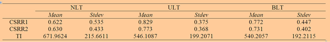
Table 1. Simulation results in the same distribution demand case

Figure 9. Total inventory in the different distribution demand case

Figure 10. Customer satisfaction rate in the different distribution demand case
4.2 Different Distribution Demand Case
We assume retailer  face different distribution demand. Retailer 1 is still subject to the Poisson distribution as described above. Retailer 2 is subject to the Normal distribution with the range from 50 units to 150 units. Simulation results are shown in Figure 9, Figure 10 and Table 2.
Comparing with that in NLT situation, the system total inventory decreases in BLT and ULT cases, but slightly. In addition, viewing the standard deviation of total inventory in three varieties of policies, we can see that it decreases slightly in the ULT, while an increase in the BLT case. It shows that transshipment is not effective with the different distribution demand case.
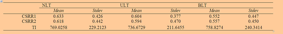
Table 2. System simulation results under different distribution of the needs
From Table 2 we can see that lateral transshipment decreases the customer demand satisfaction rate in different levels, especially the BLT. In NLT, ULT and BLT, mean of  are 0.633, 0.604 and 0.552, respectively; mean of
  are 0.618, 0.594 and 0.557, respectively. From this point, we deduce that lateral transshipment may be not compatible with the different distribution demand.
5. Conclusions
Taking the supply chain system that includes a supplier and two retailers as the research objects, this paper study the influence of lateral transshipments policy on supply chain performance based on system dynamics. We established NLT model, ULT model and BLT model. Through the simulation analysis of these three different models of the supply chain system by Venple, we found that: first, if the two retailers are facing the same distribution demand, lateral transshipments not only reduce total inventory but also increase the customer demand satisfaction rate. Moreover, the effect is more obvious in ULT case; secondly, if the two retailers are facing with the different distribution demand, lateral transshipments reduce total inventory of the system, but the extent is not obvious. However, it decreases the customer demand satisfaction rate of the supply chain system.
As to the first conclusion of this paper, we believe that lateral transshipments make the system handle inventory rationally. It decreases the total inventory, and improves customer demand satisfaction rate. It is an inventory control policy that is worth popularizing. For the second conclusion, we question the suitability of the lateral transshipments policy under the different distribution demand. The main reason may be that different distribution demand will make ordering and replenishment become extremely complex. Moreover, if the retailers still use a separate order-up-to policy, lateral transshipments may becomes impossible and difficult to improve system performance. Hence, considering lateral transshipment, how to find the optimal inventory control policy rather than simply use order-up-to policy in different distribution case will be our further research problems.
6. Acknowledgment
This paper was support, in part, by the Nantong University Social Science Foundation (No.09W021).
REFERENCES
- G. Tagaras and M. A. Cohen, “Pooling in two-location inventory systems with nonnegligible replenishment lead times,” Management Science, Vol. 38, pp. 1067–1083, 1992.
- K. S. Krishnan and V. R. K. Rao, “Inventory control in n warehouses,” Journal of Industrial Engineering, Vol. 16, pp. 212–215, 1965.
- L. W. Robinson, “Optimal and approximate policies in multiperiod, multilocation inventory models with transshipment,” Operations Research, Vol. 38, pp. 278–295, 1990.
- H. L. Lee, “A multi-echelon inventory model for repairable items with emergency lateral transshipments,” Management Science, Vol. 33, pp. 1302–1316, 1987.
- S. Axsäster, “Modelling emergency lateral transshipments in inventory systems,” Management Science, Vol. 36, pp. 1329–1338, 1990.
- T. W. Archibald, S. A. E. Sassen, and L. C. Thomas, “An optimal policy for a two depot inventory problem with stock transfer,” Management Science, Vol. 43, pp. 173–183, 1997.
- J. Grahovac and A. Chkkavarty, “Sharing and lateral transshipment of inventory in a supply chain with expensive low-demand items,” Management Science, Vol. 47, pp. 579–594, 2001.
- A. Kukreja, C. P. Schmidt, and D. M. Miller, “Stocking decisions for low-usage items in a multilocation inventory system,” Management Science, Vol. 47, pp. 1371–1383, 2001.
- N. Rudi, S. Kapur, and D. F. Pyke, “A two-location inventory model with transshipment and local decision making,” Management Science, Vol. 47, pp. 1668–1680, 2001.
- S. Minner, E. A. Silver, and O. J. Robb, “An improved heuristic for deciding on emergency transshipments,” European Journal of Operational Research, Vol. 148, pp. 384–400, 2002.
- K. Xu, P. T. Evers, and M. C. Fu, “Estimating customer service in a two-location continuous review inventory model with emergency transshipments,” European Journal of Operational Research, Vol. 145, pp. 569–584, 2003.
- A. Banerjee, J. Burton, and S. Banerjee, “A simulation study of lateral shipments in single supplier, multiple buyers supply chain networks,” International Journal of Production Economics, Vol. 81–82, pp. 103–114, 2003.
- T. Xu and S. Luo, “The expected total cost method of lateral transshipment in a cross-docking system with stochastic demand,” Industrial Engineering and Management, Vol. 9, pp. 27–31, 2004.
- T. Xu and H. Xiong, “The method of searching the best time for one-off transshipment in a cross-docking system with stochastic demand,” Systems Engineering, Vol. 22, pp. 23–26, 2004.
- Y. Wang, F. Lang, and X. Li, “The quantitative analysis on value of lateral transshipment strategy in system of inventory distribution,” Journal of Heilongjiang Institute of Technology, Vol. 20, pp. 1–5, 2006.
- J. Huo and H. Li, “Batch ordering policy of multilocation spare parts inventory system with emergency lateral transshipments,” Systems Engineering Theory & Practice, Vol. 27, pp. 62–67, 2007.
- J. Li, B. Li, and C. Liu, “Across-chain inventory management in cluster supply chains based on systems dynamics,” Systems Engineering, Vol. 25, pp. 25–32, 2007.
- F. Olsson, “An inventory model with unidirectional lateral transshipments,” European Journal of Operational Research,”, in press.
- D. Vlachos, P. Georgiadis, and E. Iakovou, “A system dynamics model for dynamics capacity planning of remanufacturing in closed-loop supply chains,” Computers and Operations Research, Vol. 34, pp. 367–394, 2007.
- J. W. Forrester, “Industrial dynamics: A breakthrough for decision makers,” Harvard Business Review, Vol. 36, pp. 37–66, 1958.
- J. D. Sterman, “Modeling managerial behavior: misperceptions of feedback in a dynamic decision making experiment,” Management Science, Vol. 35, pp. 321–339, 1989.
- S. M. Disney, A. T. Potter, and B. M. Gardner, “The impact of vendor managed inventory on transport operations,” Transportation Research Part E, Vol. 39, pp. 363– 380, 2003.
- A. C. Marquez, C. Bianchi, and J. N. D. Gupta, “Operational and financial effectiveness of e-collaboration tools in supply chain integration,” European Journal of Operational Research, Vol. 159, pp. 348–363, 2004.
- Y. Zhong, X. Jia, and X. Li, “Systems dynamics,” Science Press, Beijing, 2007.