Journal of Geographic Information System
Vol. 4 No. 2 (2012) , Article ID: 18768 , 11 pages DOI:10.4236/jgis.2012.42019
Spatial Interpolation Applied a Crustal Thickness in Brazil
1Seismological Observatory, University of Brasilia, Brasília, Brazil
2Laboratory of Remote Sensing and Spatial Analysis, University of Brasília, Brasília, Brazil
Email: cesargarciapavao@gmail.com.br
Received December 15, 2011; revised January 28, 2012; accepted February 16, 2012
Keywords: Spatial Interpolation; Crustal Thickness; Tectonic Provinces of Brazil
ABSTRACT
The use of spatial interpolation methods of data is becoming increasingly common in geophysical analysis, for that reason, currently, several software already contain many of these methods, allowing more detailed studies. In the present work four interpolation methods are evaluated, for the crustal thickness data of Brazil tectonic provinces, with the intention of making Moho’s map of the regions. The methods used were IDW, Natural Neighbor, Spline and Kriging. We compiled 257 data that constituted a geographic database implemented in the template Postgree PostGIS and were processed using the tools of interpolation located in the Spatyal Analyst Tools program ArcGIS®9 ESRI. Traditional methods, IDW, Natural Neighbor and Spline, generate artifacts in their results, the effects of aim, not consistent with the behavior of crust. Such anomalies are generated because of mathematical formulation methods added to data compiled gravimetry. The analysis results of geostatistical Kriging are more refined and consistent, showing no specific anormalities, i.e., the crustal thickness variation (thinning and thickening) is introduced gradually. Initial our estimates were separated in four specific blocks. With the approval of new networks (BRASIS, RSISNE and RSIS), the crustal thickness database for Brazil may be amended or supplemented so that new models may be generated more consistently, complementing studies of regional tectonics evolution and seismicity.
1. Introduction
Advancements in computing, development of geophysical methodologies and improvements in mapping techniques that are taking place recently have provided us means for a more precise evaluation of mapped aspect’s quality, as well as means for a scrutiny aiming to detect errors associated to them, which can be caused at the moment of determining the spatial representation model. In these circumstances, there was a necessity of implementing methods for spatial interpolation of data in geographic information systems, more sophisticated ways of producing, analyzing, and interpreting information, allying them with proceedings for evaluating trustability and significance of the results.
According to [1], interpolation is the mathematical process for finding intermediate values among a function’s discrete values. [2] defines the spatial interpolation more specifically, as a proceeding for estimating nonsampled local propriety values, basing on values of data observed in known places. [3] provides a didactic classification through different viewpoints. The interpolators are classified as global or local, exact or softening, deterministic or stochastic. The global functions consider all the area points and permit to interpolate the value of the function in any other point inside the domain of the original data, and the addition or subtraction of a value will result in the domain of the function definition. In the other hand, the local functions are defined for portions of the map, and the alteration of a value will locally affect the points close to it.
Exact interpolations are normally used when the values of the points in which the interpolation is based are precise. In this case, there is not the presence of residuum, that is to say, prediction on sampled localities will equal the sampled value [4]. In the other hand, softening interpolates are used when there is uncertainty on the sampled values. They soften the curves of the generated surface and minimize data errors.
Stochastic interpolates make use of the probability theory and incorporate statistical criteria for determining the relevance attributed to the sampled points in order to calculate the interpolations. Deterministics do not make use of statistic methods for calculating the measure of a scalar in space. They make a linear combination of sampled values, basing on the spatial distribution geometry of the sampled points [5].
Due to the variety of available interpolation methods, the selection of the most appropriate one for each individual case is pertinent [6,7]. [8] affirms that there is no statistic theory that is able to indicate which interpolation technique is superior. There is no simple response when someone deals with the choice of a superior or proper spatial interpolator. This depends on plenty of variables, such as the spatial configuration of data and the parameters to be studied [9]. According to [10], each spatial interpolation method can be efficient for a specific use, which depends on the phenomenon to be studied. There are few references to studies on spatial interpolation methodologies. [11,12] assert that other authors have made a general approach of methods in research areas like soil science, meteorology, hydrology, and forestry. Nevertheless, a more precise method is not defined yet.
In this context, this work’s objective is to evaluate comparatively four spatial interpolation methods for crustal thickness data of Brazilian tectonic provinces. The best way of representing spatially this variable, the effective resolution of the fact that the more quoted global models [13,14] are under the formal resolution in consequence of seismic data deficiency in large regions like South America [15] and the non-description of proceedings for their production have motivated the development of this work.
2. Area of Study
Once Brazil is a country that has a continental dimension, [16,17] applied the concept of structural provinces. This concept had already been implemented in other countries such as Canada and Australia, taking into consideration that structural provinces present their own magmatic, metamorphic, stratigraphic and tectonic features, and they are different from the nearby provinces.
The province’s limit is geologically defined by faults, fault zones, metamorphic fronts, foreland zones, erosional limits of sedimentary areas. Figure 1 presents a subdivision of Brazil in structural provinces in the perspective of Brazilian Geological Service [18]. According to this figure, Brazil is divided in eight large structural provinces: Borborema Province (1), Tocantins Province (2), Paraná Basin (3), Mantiqueira Province (4), Northern Amazon Craton (5), Parnaíba Basin (6), Southern Amazonas Craton (7), and São Francisco Craton (8). Readers can find information on the Brazilian structural provinces in [16,18-25].
3. Material and Methods
3.1. Data
Recent developments of geophysical methodologies such as the receiver function have made possible some advancement in the crustal structure studies in Brazil. In this context, 257 crustal thickness points were compiled through the receiver function, both seismic and gravimetric
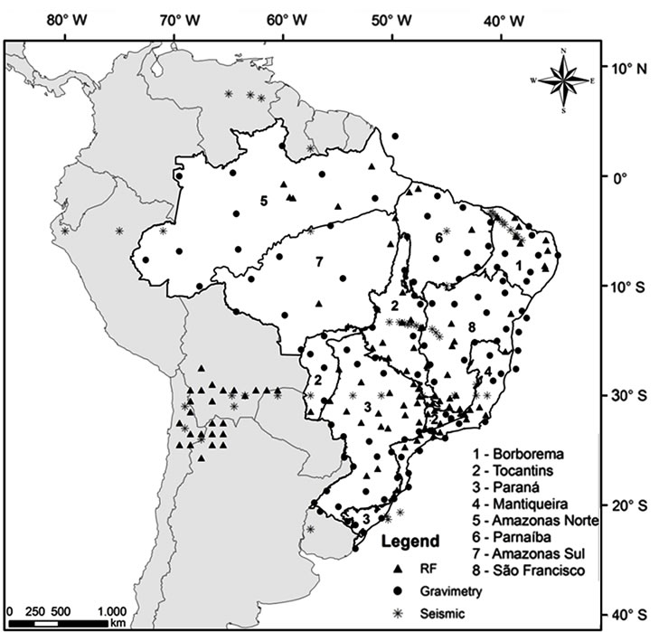
Figure 1. Division of Brazilian territory in structural provinces according to Brazilian Geological Service (Modified Bizzi et al. 2003). The triangles represent crustal thickness values obtained through the receiver function, the asterisks obtained through seismic, and the circles obtained through gravimetry.
estimate (Figure 1). Table 1 organizes data by authors and methodologies. Inside the total amount, 206 points are in Brazilian inlands. The other ones were used in order to minimize border errors in the interpolation process (Figure 1). Due to be a large portion of the land surface, located in South America, for this work, we used geodetic coordinates of the Cartesian reference system Topocentric of South America 1969 (datum SAD69), usual system in Brazil where spatial information are from the 1970s. For defining interpolation parameters, an analysis was made in order to check the distribution of crustal thickness points.
The distance from the centroid of each point to the centroid of the nearby points was calculated. If the average distance has a value that is inferior to the average for a hypothetical aleatory distribution, the distribution of the analyzed thickness points is considered as grouped. And if the average distance is larger than the average for a hypothetical aleatory distribution, the characteristics are dispersed. The relation used in the analysis is defined by:
 (1)
(1)
where Do is the average distance observed between each point and its closest neighbor, and De represents the average distance expected for the points in an established aleatory standard and defined respectively by:
 (2)
(2)

Table 1. Compilation of crustal thickening data obtained through the receiver function, seismic, and gravimetry as they were used in this work. It is organized by author and method.
 (3)
(3)
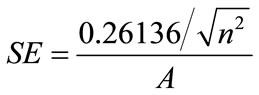
where d is the distance amid a fixed point and its neighbors, n corresponds to the total number of points, and A is the total area of study. The percentage (%) of Z-score is calculated by:
 (4)
(4)
where:
 (5)
(5)
According to the analysis, the conclusion is that the crustal thickness data are presented randomly in 95%, that is, they are disposed in an aleatory way, and the average distance among the points is 1474.81 km.
3.2. Interpolation Methods
A decision was taken to work with only one software (ArcGis®9 ESRI) and also to adopt its nomenclatures for the interpolation methods. They can vary in accordance to software and authors. The methods used are presented in details and with mathematical rigor according to ESRI, and they can be briey described like this:
1) Inverse Distance Weighting (IDW): IDW determines values of cells using a linear pondered combination of sampled points assemblage. This method can be classi_ed as an exact interpolator, as well as a softener. This method attributes a major weight to the closest point, diminishing this weight while distance gets larger, that is, the heavier the weight, the smaller the inuence of the most distant points from the knot. Details on this method were well-described by [49].
2) Natural Neighbor: Natural Neighbor method is a local interpolator that relates to an entrance sample subgroup to a point of consultation and apply weights to them, basing on proportional areas, that is to say, interpolation is done through the nearby points pondered average in which weights are proportional to proportional areas. This is a different technique, once it does not extrapolate values, resolving the interpolation only inwards data domain. Details on this method were well-described by [50,51].
3) Spline: Spline method does not use only one big grade polynomial for interpolation of all data group. The technique divides a data series in subgroups and uses several small grade polynomials for each subgroup. The method is classified as a softener and tries to do credit to the data at its maximum. In this process, derivation calculi are repeatedly done up to the reach of a diference (convergence or tolerance) amidst sampled or estimated values. It is specified by the user or it is done up to the reach of the maximum number of iteration. The method can produce local artifacts of excessively high or low values [52]. Details on this method were well-described by [53,54].
4) Kriging: Kriging is a stochastic interpolator that can present characteristics of an exact interpolator or a softener. The method uses geostatistics for executing interpolation. The word “geostatistics” is relatively recent. It was designated by Matheron in his work for solving spatial problems related to mining [55]. This technique is based on a function that explains a variables behavior in different directions in a geographic space. It also permit to associate the estimation variability based on the distance between a pair of points using semivariograms which permit to check the dependence level or the spatial correlation amidst samples [6]. The method requires at least 100 sampled points in order to produce a trustworthy estimate of the variogram [56]. The spherical variogram model with nugget was used where the nugget is 9.40, the sill is 88.88 and range is 44.65. Details on this method were well-described by [2,57-61].
4. Results and Discussions
Interpolations were executed for each method, using resolution grids of 104 × 105, 130 × 131, 174 × 175, 260 × 261, and 524 × 525 lines by column. Once the sampled region is more latitudinally extended, the line number differs from the column number in order to force square meshes which minimize distortions in interpolations. In the other hand, rectangular meshes tend to produce anisotropic effects in the results [4]. These grids represent exit pixels of approximately 41.70 km, 33.25 km, 24.90 km, 16.70 km and 8.30 km respectively.
For a comparison of interpolation methods, the exit pixel of 16.70 km is used, once there is not a set up theory for defining the grid size to be used. A mesh that contains more than one sampled point inside a square tends to minimize features with physical significance of interest. In case of a dense grid, the interpolator can create more values amidst the sampled points, which can cause unreal tendencies in the results [4]. However, it is possible to establish a proportionality scale between half of the distribution space length of the sampled points and the interpolation grid.
The average distance amidst the crustal thickness points was 1474.81 km. The sampled space has a latitudinal length of 4403.50 km and a longitudinal length of 4386.85 km. So, the grid resolution that get closer to the established proportion is 260 × 261 (pixel of 16.70 km) Figure 2, line by column, respectively. Besides the crustal thickness spatial distribution maps, residues and the difference between the calculated value and the observed value were calculated. From residues, Mean Error (ME), Mean Square Error (MSE), Root Mean Square Error (RMSE) and Model Efficiency (EF) were also calculated.
The closer to 1 is the EF value, the more efficient the method is. If EF tends to zero, this indicates that the average value of the observations is more trustworthy than the estimated ones and the model has limitations [62]. Table 2 shows the values of ME, MSE, RMSE and EF obtained for the four analyzed methods.
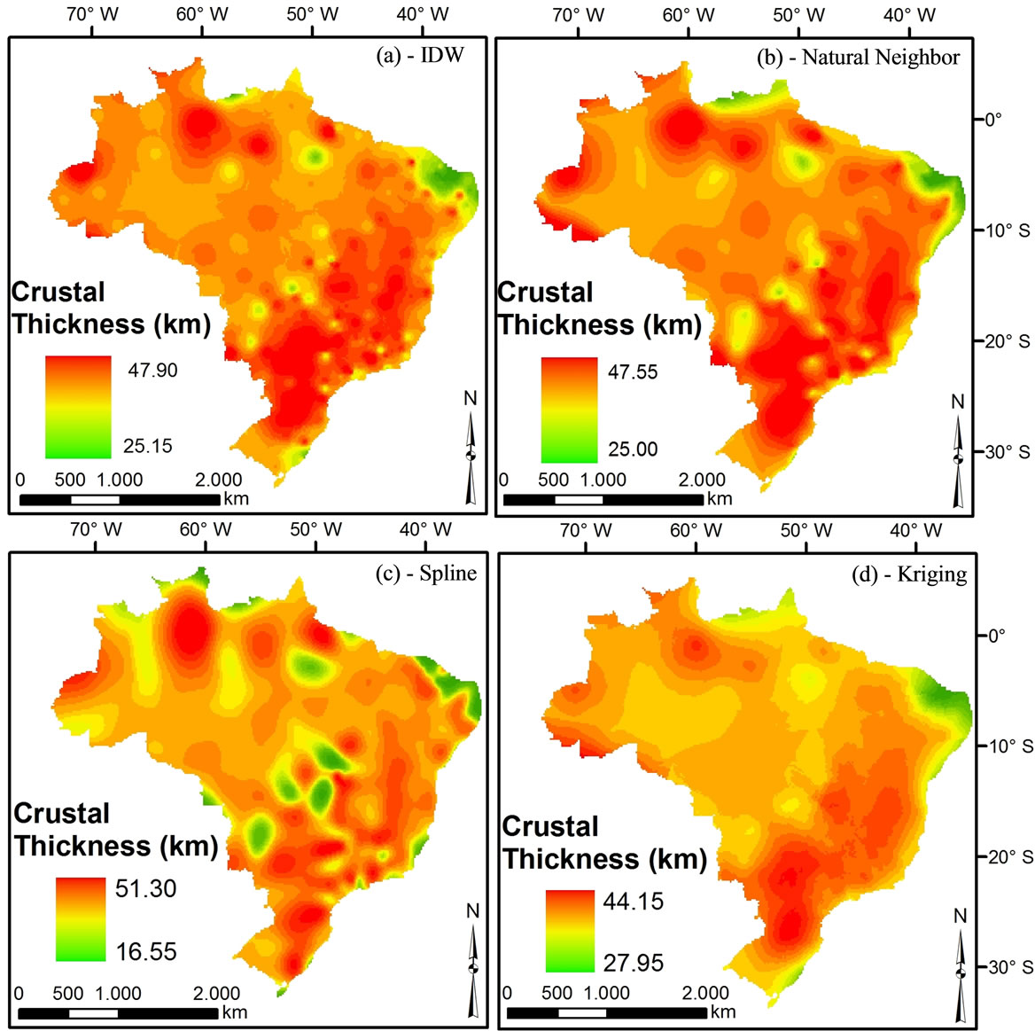
Figure 2. Results of spatial interpolation for crustal thickness data using the following methods: (a) IDW; (b) Natural Neighbor; (c) Spline and (d) Kriging for exit pixel of 16.70 km (mesh 260 × 261 lines by column, respectively).
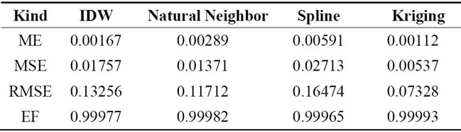
Table 2. Measurements used to assess the performance of the spatial interpolation methods. Where ME = Mean Error, MSE = Mean Square Error, RMSE = Root Means Square Error and EF= Model Efficiency.
Amidst the analyzed methods, Kriging has resulted in closest to zero ME and MSE values, and a smaller RMSE value. For the Efficiency Model (EF), the methods have presented close to 1 values. Receiver function is a geophysical technique that seeks punctually infers information on Earths internal structure, measuring more precisely the thickness of the mantle crust. In this technique, an error of ±1.00 km in the calculated value of the crustal thickness is admitted. So, this margin was used for comparison between models obtained without preoccupation with the technique used in the crustal estimate. Figure 3 presents the graph of error x calculated, and the linear regression for every analyzed method: (a) IDW; (b) Natural Neighbor; (c) Spline and d) Kriging.
The models obtained through IDW methods (a) and Natural Neighbor (b) have similar characteristics. Bull’s eye effect was observed in both of them, and the IDW was in larger quantity. Both methods have shown minimum thickness (~25 km) and maximum thickness (~48 km), according to the entry data. IDW has presented 86 thickness calculated values above the established limit, and the Natural Neighbor has presented 62 values (Figure 3). These error values are justified by the absence of crustal thickness data in the Brazilian coast (Atlantic Ocean), generating border errors in the interpolation processes. The model generated by the Spline method (c) produces artifacts that do not represent the crust physical characteristics. This can be observed in Central Brazil. The other three methods present a crust without abrupt variation, except bull’s eye effect (IDW and Natural Neighbor). The Spline method (c) presents three adjustment anomalies and a crustal thickening in this region. [45] have estimated through the deep refraction seismology the crustal thickness of this region. It varies from 36 to 44 km. On the other hand, the Spline method (c) has calculated values from approximately 17 to 51 km to the same region. From the four models evaluated, Spline (c) presented a larger error quantity (125), being above the established limit, and the major maximum error (3.47 km) (Figure 3).
The crustal thickness map generated by the Kriging method (d) has presented the smaller error quantity (1) above the limit of ±1.00 km and the smaller maximum error value (1.09 km) (Figure 3). The largest error values for this method, as well as the model generated by Spline,
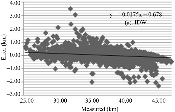
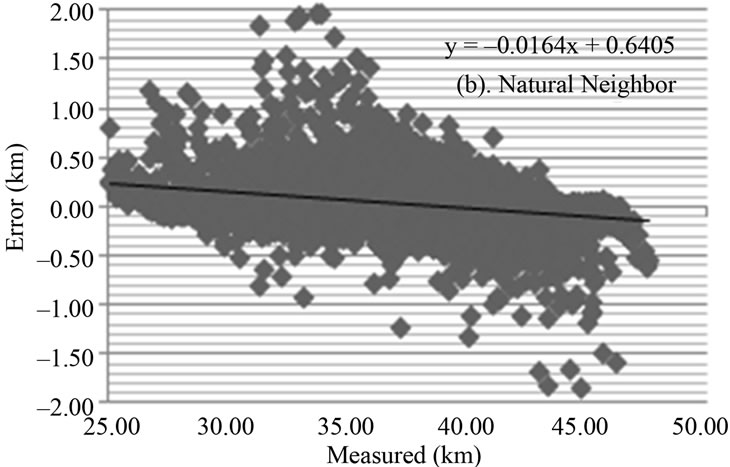
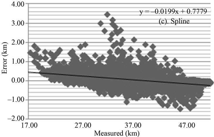
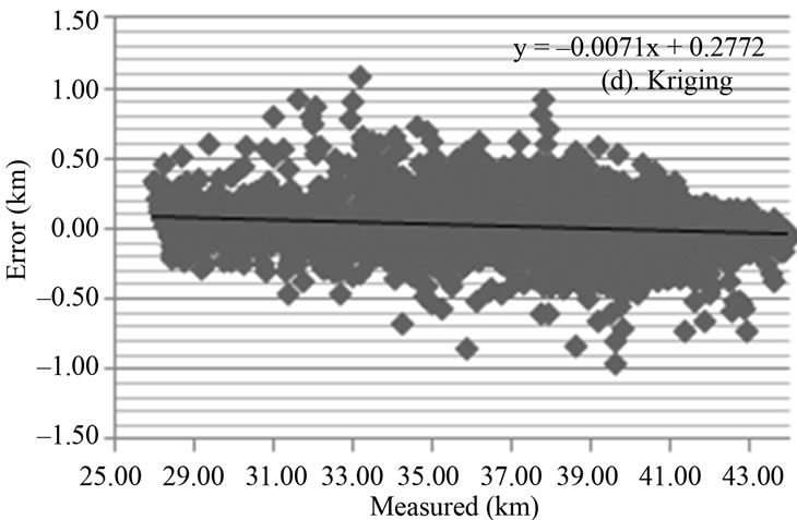
Figure 3. Graphs error X calculated for the spatial interpolation method (a) IDW; (b) Natural Neighbor; (c) Spline and (d) Kriging, linear adjustment for each method.
are border errors in the east coast of Brazilian territory. In general, the model presents crustal thickness variations, sharpening and thickening. They are gradual, more consistent with the crust physical characteristics.
For a comparison of each two of the models, a subtraction was made amidst the models generated by the four interpolation methods, emphasizing the studied portions of the territory that present larger discrepancies between the calculated values for each method (Figure 4).
The limit error of ±1.00 km was maintained for an analysis and to make contrasts in the results evident. The results within the error limit are in green, and the results above the limit are in red. The operations using Spline method (iii, v, vi) have produced a large quantity of results above the established error limit, in red. This can be explained by the maximum values and by the fact that the minimum calculated through this method does not reach the exit data. The subtraction result of the IDW method by the Natural Neighbor (ii) has produced beyond the pre-established error limit results in small portions of the area, the predominant green class, and the similarity of the minimum and maximum values obtained through methods that define a similarity in models generated by them. Item (i) in Figure 4, subtraction amidst IDW and Kriging methods, characterize bulls eye effect produced by the IDW, taking into consideration that Kriging does not produces this kind of artifact.
The average of residues in function of diminishing the model resolution for each method is represented in Figure 5.
With the exception of the model generated by Spline method, the largest values are associated with the smallest resolutions (largest exit pixels). Method IDWpresents an increase in the error average as the model resolution diminishes. The models generated by Spline method present errors of approximately 10–3, with the exception of a grid with a pixel of 16.70 km. The curves that represent Natural Neighbor and Kriging models behave the same way, and the error average of Natural Neighbor method is superior to the one of Kriging method.
The residue’s variance (Figure 6) shows that Natural Neighbor, Spline and Kriging methods present similar behavior, with larger values for smaller resolutions. These values diminish according to the increase of them, tending to zero. Spline method for pixel resolutions of 24.90 km, 33.25 km and 41.70 km presents variance values that are superior to the ones for Natural Neighbor and Kriging methods. The largest value of all the mentioned method was approximately 1.2 for Spline in the pixel grid of 41.70 km.
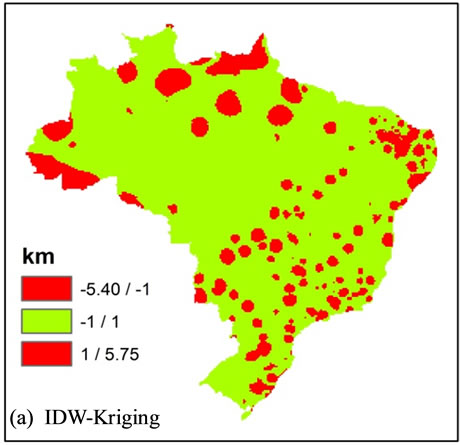
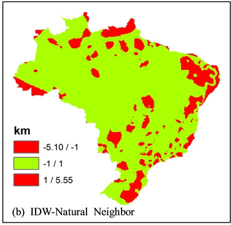
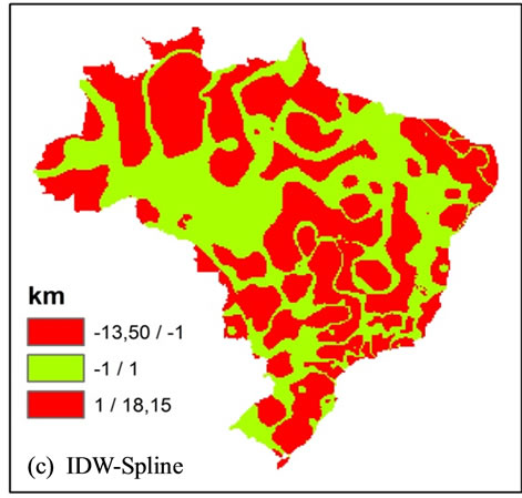
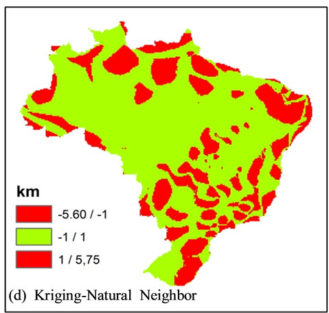
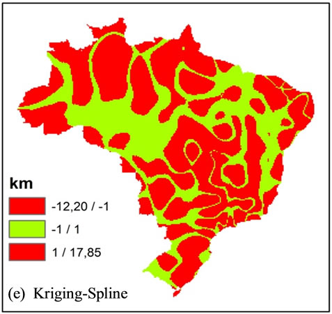
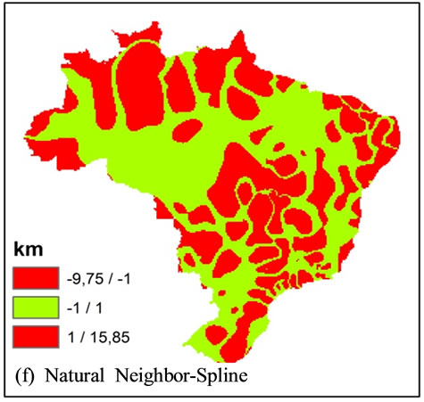
Figure 4. Comparison between the obtained models. In (a) Subtraction between the models IDW and Kriging; (b) Subtraction between IDW and Natural Neighbor; (c) Subtraction between IDW and Spline; (d) Subtraction between Kriging and Natural Neighbor; (e) Subtraction between Kriging and Spline and (f) Subtraction between Natural Neighbor and Spline. Values above the established error limit is in red, and values within the error limit is in green (±1.00 km).
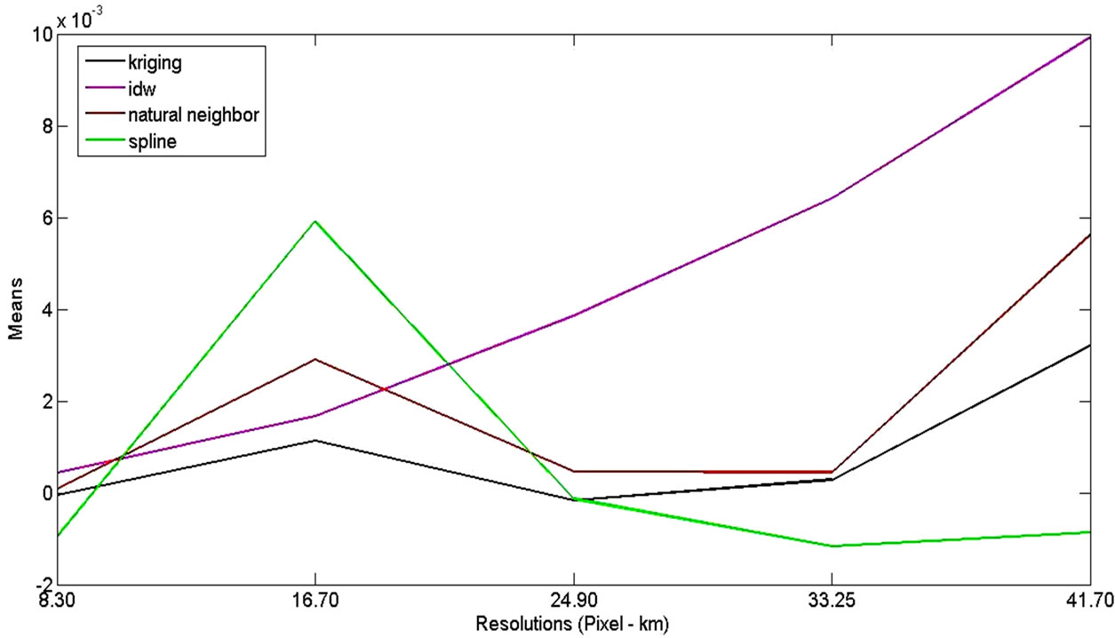
Figure 5. Variation of residues average in function of the mesh resolution (pixel km) for the interpolation methods used.
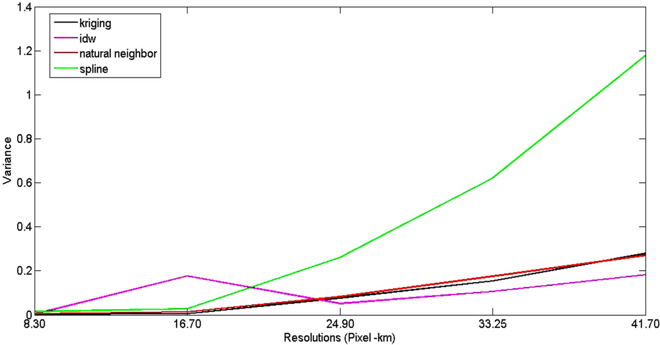
Figure 6. Variation of the residues variance in function of the mesh resolution (pixel km) for the interpolation methods used.
General standard of residual behavior of interpolations aimed to minimize variance through the increase of mesh resolution, being in accordance to the observed data. Figure 6 shows that a larger reduction, in general terms, occurs between resolutions of 41.70 km and 24.90 km. Even with the resolution increase, there are no significant improvements in the results. An effective comparison to show which method generates better interpolations is subjective, once, as [8] wrote, there are no statistical tests for proving interpolation efficiency. Therefore, it is more suitable to determine which methods have presented results that were more coherent with the reality of the phenomenon in study. Our option for Kriging method occurred because it presents a smaller error quantity beyond the limit: ±1.00 km. Figure 7 illustrates the effect of diminishing resolution using Kriging method. It was more suitable for representing crustal thickness in Brazil (Figure 2). Largest changes take place between the resolutions 24.90 and 16.70. Its main effect is a model softening.
As long as this is a subjective analysis, a visual comparison was done using Crust 2.0 worldly scale model [14]. This model is an updating of Crust 5.1 [13]. It is specified in a grid scale of 2 × 2 grades. The value compilation of the crustal thickness covers the major part of Eurasia, North America, Australia, and the Andes. Besides the crustal thickness, this model permits to infer information
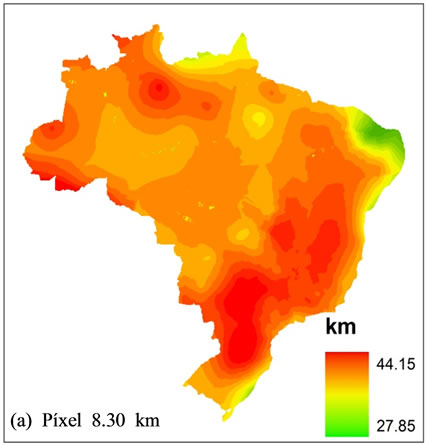
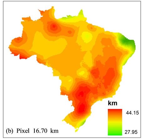


Figure 7. Results of crustal thickening interpolation data, using Kriging method for different resolutions.
on ice layers, sedimentary layers, superior crust, and inferior crust. Information on Vp and Vs are explicitly given for all the model layers. Figure 8 shows Crust 2.0 model and the model obtained by Kriging method with a pixel of 16.70 km. It is important to emphasize that a cutout of Crust 2.0 model was done in Brazils region, and the same subtitle was maintained, varying approximately from 0 to 70 km. It was used for the whole model. Crust 2.0 model presents basically three thickness values for the Brazilian territory. A value represented by the dark green class (~25 - 30 km) in the east border indicates a crustal sharpening in the direction of the Atlantic Ocean.
This feature is also observed in the Kriging model. A light green class includes the provinces described in Figure 1: Borborema (1), São Francisco Craton (8), Mantiqueira (4) and part of Tocantins (2), Parnaíba (6), Amazon Craton (5) and Paraná Basin. This class represents a thickness between 33 and 38 km approximately. The third class is represented by the yellow color and its thickness is approximately between 39 and 45 km. It contains the major part of Amazon Craton (5, 7), Paraná Basin (3), as well as the resting part of Tocantins Province (2). The model generated by Kriging shows a better definition of the crustal structure for Brazil. It is possible to observe a gradual thickness variation within the same tectonic province. This fact is due to the number of crustal
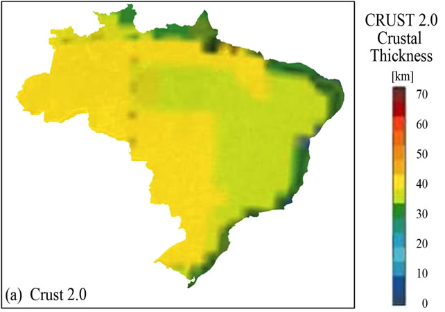
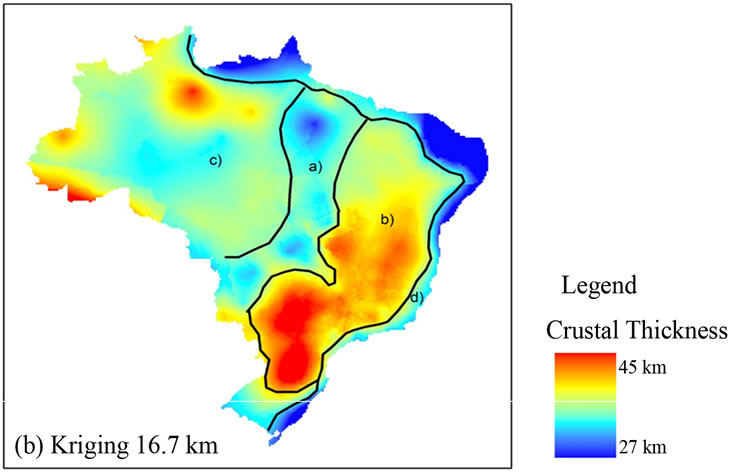
Figure 8. Comparison between model (a) Crust 2.0 (Modified [14]) and (b) model obtained by Kriging, with resolution of 16.70 km.
thickness values that are compiled for generating each model, considering that Crust 2.0 model presents a deficiency in data compilation in both the African and the South American continent. The model obtained by Kriging has 257 thickness values.
The entry data of Crust 2.0 are all proceeding from a seismic, and the data of the model generated by Kriging are obtained through a seismic, function of receiver and gravimetry. The methodologies of the receiver function and the seismic are efficient for calculating crustal thickness, and gravimetry provides a relative response using a priori information. The work of [26] considered two models for calculating crustal thicknesses that are compatible with the demands of isostasy. The first model admitted a smaller density of lithospheric mantle in the craton area and the second larger crustal density of Paran Basin. 104 crustal thickness data obtained by gravimetry were used for the models got through this work. Despite of these data present a smaller precision than the ones of the seismic data and receiver function, they were very important for occupying portions of the territory on which there were not information about the other two methods, as well as for minimizing errors in Brazil’s east border.
Our estimates were separated in four specific blocks:
1) Central sharpening: This result shows a crust that raises and sharpens in Brazilian interplate.
2) Crustal thickening: The thickest crust region. It contains So Francisco Craton and Paraná Basin, regions with less seismic activities than other parts of the country.
3) Initial estimate: Region with smaller quantity of information. Nevertheless, some estimates show a larger thickness at the north part and an intermediate thickness at the central and south area. This demonstrates that the crust suffers effects of tectonic collision or separation.
4) Marginal sharpening: With the crustal thickness estimates in NE by Receiver Function, it is possible to realize that in this region the crust sharpens towards the continental margin.
5. Conclusions
Resolutions of interpolation mesh must be coherent with the sampled mesh resolution. Therefore, a great computational effort for interpolation through exit pixel diminishing do not necessarily generates the best results. Seismic data, receiver function and gravimetry like they were compiled for this work were efficient for repre-senting the crustal thickness of Brazilian tectonic provinces. From the four methods evaluated for a spatial representation of the crustal thickness, Kriging method produced the best results, even if in regions like Amazon Craton (5.7) they do not present the gradual behavior of the expected sharpening/thickening for Earth’s crust. This fact is explained by the reduced number of thickening data in that region. In their major part, they are gravimetry data.
With the implement of the geographic database of Brazil’s crustal thickening, it can be updated whenever new studies on the crustal thickness of this region are published. After the verification of Kriging spatial interpolation method as the most efficient for crustal thickness data, new models for crust depth for Brazils structural provinces can be generated in a practical, quick and efficient way.
6. Acknowledgments
The authors thank the Laboratory of remote sensing and spatial analysis (LSRAE) IG/UnB scholarship by providing a technique for the first author during the development of his doctorate. ESRI for providing the package of tools that make up the through ArcGIS 10 family of the contract number 2011 MLK 8733 and a IMAGEM for the support and feasibility of establishing the terms of use and between the IG and the support of ESRI software.
This research is supported CNPq/Instituto do Milênio grant 420222/05-7 and CNPq/INCT 573713/2008-1. We special thank all technicians from UnB, USP and UFRN, for their efforts in the field work, maintenance of equipment, and preliminary readings of data. GSF thank CNPq for their PQ grants. Adriano Rabelo for improvement of the English.
REFERENCES
- P. Stark, “Introdução aos Métodos Numéricos; Interciência,” Tradução de João Bosco Pitombeira de Carvalho, Rio de Janeiro, 1979.
- P. A. Burrough, “Principals of Geographical Information Systems for Land Resources Assessment,” Clarendon Press, Oxford, 1986.
- A. D. Hartkamp, K. De Beurs, A. Stein and J. W. White, “Interpolation Techniques for Climate Variables,” NRGGIS Series 99-01, CIMMYT, Mexico City, 1999, pp. 1-34.
- P. L. F. Mazzini and C. A. F. Schettini, “Avaliação de Metodologias de Interpolação Espacial Aplicadas a Dados Hidrográficos Costeiros Quase Sinóticos,” Brazilian Journal of Aquatic Science and Technology, Vol. 13, No. 1, 2009, pp. 53-64.
- A. Soares, “Geoestatística Aplicada a Ciências da Terra e do Ambiente,” IST Press, Lisbon, 2000.
- N. Cressie, “Statistics for Spatial Data,” John Wiley & Sons Inc., New York, 1991.
- E. J. Englund, “A Variance of Geostatisticians,” Mathematical Geology, Vol. 22, No. 4, 1990, pp. 417-455. doi:10.1007/BF00890328
- J. C. Davis, “Statistics and Data Analysis in Geology,” 2nd Edition, John Wiley and Sons Inc., New York, 1986.
- E. H. Isaaks and R. M. Srivastava, “Applied Geostatistics,” Oxford University Press, New York, 1989.
- C. Childs, “Interpolating Surfaces in ArcGIS Spatial Analyst,” ArcUser, 2004, pp. 32-35.
- M. A. Aguilar, F. J. Aguilar, F. Carvajal and F. Aguera, “Evaluación de Diferentes Técnicas de Interpolación Espacial Para la Generación de Modelos Digitales de Elevación del Terreno Agrícola,” Mapping, No. 74, 2001, pp. 72-92.
- C. R. Mello, J. M. Lima, A. M. Silva, J. M. Mello and M. S. Oliveira, “Krigagem e Inverso do Quadrado da Distância Para Interpolação dos Parâmetros da Equação de Chuvas Intensas,” Revista Brasileira De Cincia De Solo, Vol. 25, No. 5, 2003, pp. 925-933. doi:10.1590/S0100-06832003000500017
- W. D. Mooney, G. Laske and G. T. Masters, “Crust 5.1: A Global Crust Model at 5˚ × 5,” Journal of Geophysical Research, Vol. 103, No. B1, 1998, pp. 727-747. doi:10.1029/97JB02122
- G. Laske, “Crust 2.0: A Global Crust Model at 2 × 2,” 1999. http://igpp.ucsd.edu/ gabi/crust2
- N. C. Sá, “O Campo de Gravidade, o Geóide, e a Estrutura Crustal na América do Sul,” Ph.D. Thesis, Universidade de São Paulo, São Paulo, 2004, 136 p.
- F. Almeida, B. Brito Neves and R. A. Fuck, “Províncias Estruturais Brasileiras,” Simpósio de Geologia do Nordeste, Vol. 8, 1977, pp. 363-391.
- F. F. M. Almeida, Y. Hasui, B. B. Brito Neves and R. A. Fuck, “Brazilian Structural Provinces: An Introduction,” Earth Sciences Reviews, Vol. 17, No. 1-2, 1981, pp. 1-29. doi:10.1016/0012-8252(81)90003-9
- L. A. Bizzi, C. Schobbenhaus, R. M. Vidotti and J. H. Gonalves, “Geologia, Tectônica e Recursos Minerais do Brasil,” CPRM, Brasília, 2003.
- F. F. Alkmim, “O que faz de CRátron um Cráton? O Cráton do São Francisco e as Revelações Almeidianas ao Delimitá-lo,” In: Geologia do Continente Sul-Americano: Evolução da Obra de Fernando Flávio Marques Almeida, Editora Beca, São Paulo, 2004.
- C. C. G. Tassinari and M. J. B. Macambira, “A Evolução Tectônica do Cráton Amazônico,” In: Geologia do Continente Sul-Americano: Evolucão da Obra de Fernando Flávio Marques de Almeida, Vol. 28, Editora Beca, São Paulo, 2004.
- B. B. Brito Neves, E. J. Santos and W. R. van Schmus, “Tectonic History of the Borborema Provincy, Northeastern Brazil,” In: Tectonic Evolution of South America, International Geological Congress, Rio de Janeiro, 2000.
- L. C. Silva, N. J. Mcnaughton, R. Armstrong, L. A. Hartmann and I. R. L. A. Fletcher, “The Neoproterozoic Mantiqueira Province and Its African Connections: A Zirconbased u-pb Geochronologic Subdivision for the Brasiliano/Pan-African Systems of Orogens,” Precambrian Research, Vol. 136, No. 3-4, 2005, pp. 203-240. doi:10.1016/j.precamres.2004.10.004
- E. J. Milani, “Evolução tectono-estratigráfica da Bacia do Paraná e Seu Relacionamento Coma Geodinâmica Fanerozóica do Gondwana Sulocidental,” Ph.D. Thesis, Universidade Federal do Rio Grande do Sul, Rio Grande do Sul, 1997.
- E. J. Milani and V. A. Ramos, “Orogenias Paleozóicas no Domínio sul Ocidental do Gondwana e os Ciclos de Subsidência da Bacia do Paraná,” Revista Brasileira de Geociências, Vol. 28, No. 4, 1998, pp. 473-484.
- E. J. Milani and A. Thomaz, “Sedimentary Basins of South America,” In: Tectonic Evolution of South America, International Geological Congress, Rio de Janeiro, 2000.
- M. Assumpção, D. James and A. Snoke, “Crustal Thicknesses in SE Brazilian Shield by Receiver Function Analysis: Implications for Isostatic Compensation,” Journal of Geophysical Research, Vol. 107, No. B1, 2002, p. 2006. doi:10.1029/2001JB000422
- S. L. Beck, G. Zandt, S. C. Myers, T. C. Wallace, P. G. Silver and L. Drake, “Crustal Thickness Variations in the Central Andes,” Geology, Vol. 24, No. 5, 1996, pp. 407-410. doi:10.1130/0091-7613(1996)024<0407:CTVITC>2.3.CO;2
- M. B. Bianchi, “Variações da Estrutura da Crosta, Litosfera e Manto Para a Plataforma Sul Americana Através de Funções do Receptor Para Ondas P e S.,” Ph.D. Thesis, Universidade de São Paulo, São Paulo, 2008.
- G. S. França and M. Assumpção, “Crustal Structure of the Ribeira fold Belt, SE Brazil, Derived from Receiver Functions,” Journal of South American Earth Sciences, Vol. 16, No. 8, 2004, pp. 743-758.
- J. E. Case, T. L. Holcombe and R. G. Martin, “Map of Geologic Provinces in the Caribbean Region,” Geological Society of America, the Caribbean-South American Plate Boundary and Regional Tectonics, 1994, pp. 1-30.
- H. K. Chang, R. O. Kowsmann, A. M. F. Figueiredo and A. Bender, “Tectonics and Stratigraphy of the East Brazil Rift System: An Overview,” Tectonophysics, Vol. 213, No. 1-2, 1992, pp. 97-138.
- D. F. Albuquerque, C. G. Pavão, R. T. G. da Silveira, I. G. dos Santos and G. S. França, “Crustal Thickness Estimatives and Vp/Vs Ratio Using Receiver Functions,” 12th International Congress of the Brazilian Geophysical Society, Rio de Janeiro, 15-18 August 2011.
- R. L. Fontana, “Geotêctnia e Sismoestratigrafia da Bacia de Pelotas Plataforma de Florianópolis,” Ph.D. Thesis, Universidade Federal do Rio Grande do Sul, Porto Alegre, 1996.
- G. S. L. A. França, “Estrutura da Crosta no Sudeste e Centro-Oeste do Brasil, Usando Função do Receptor,” Ph.D. Thesis, University of São Paulo, São Paulo, 2003.
- Y. Fukao, A. Yamamoto and M. Kono, “Gravity Anomalies across the Peruvian Andes,” Journal of Geophsical Research, Vol. 94, No. B4, 1989, pp. 3890-3897. doi:10.1029/JB094iB04p03867
- P. Giese and J. Schutte, “Preliminary Report on the Results of Seismic Measurements in the Brazilian Coastal Mountains in March/April 1975,” Technical Report, University of Berlin, Berlin, 1975.
- F. Kruger, F. Scherbaum, J. W. C. Rosa, R. Kind, F. Zetsche and J. Hohne, “Crustal and Upper Mantle Structure of the Amazon Region (Brazil) Determined with Broadband Mobile Stations,” Journal of Geophysical Research, Vol. 107, 2002, p. 2265. doi:10.1029/2001JB000598
- L. S. Lloyd, S. Van der Lee, G. S. França and M. F. M. Assumpção, “Moho Map of South America from Receiver Functions and Surface Waves,” Journal of Geophysical Research, Vol. 115, 2010, p. B11315. doi:10.1029/2009JB006829
- M. S. M. Mantovani, A. Vasconcelos and W. Shukowsky, “Brusque Transect from Atlantic Coast to Bolivian Border, Southern brazil,” Vol. 4, AGU, Washington DC, 1991. doi:10.1029/GT004
- R. M. D. Matos, “The Northeastern Brazilian Rift System,” Tectonics, Vol. 11, No. 4, 1992, pp. 766-791. doi:10.1029/91TC03092
- M. F. Novo Barbosa, “Estimativa da Espessura Crustal na Província Borborema (NE-Brasil) Através de Função do Receptor,” Master’s Thesis, University Federal of Rio Grande do Norte, Natal, 2008.
- R. G. Oliveira, “Arcabouço Geofísico, Isostasia e Causas do Magmatismo Cenozóico da Província Borborema e de sua Margem Continental (Nordeste do Brasil),” Ph.D. Thesis, University Federal of Rio Grande do Norte, Natal, 2008.
- C. G. Pavão, “Estudo de Descontinuidades Crustais na Província Borborema usando a Função do Receptor,” Master’s Thesis, University of Brasília, Brasilia, 2010.
- M. Schmitz, D. Chalbaud, J. Castillo and C. Izarra, “The Crustal Structure of the Guayana Shield, Venezuela, from Seismic Refraction and Gravity Data,” Tectonophysics, Vol. 345, No. 1-4, 2002, pp. 103-118. doi:10.1016/S0040-1951(01)00208-6
- J. E. Soares, J. Berrocal, R. A. Fuck, W. D. Mooney and D. B. R. Ventura, “Seismic Characteristics of Central Brazil Crust and upper mantle: A Deep Seismic Refraction Study,” Journal of Geophysical Research, Vol. 111, 2006, p. B12302. doi:10.1029/2005JB003769
- N. Ussami, N. C. Sa and E. C. Molina, “Gravity Map of Brasil. 2. Regional and Residual Isostatic Anomalies and Their Correlation with Major Tectonic Provinces,” Journal of Geophysical Research, Vol. 98, No. B2, 1993, pp. 2199-2208. doi:10.1029/92JB01398
- R. M. Vidotti, “Lithospheric Struture beneath the Paran and Paran Basins, from Regional Gravity Analyses,” Ph.D. Thesis, The University of Leeds, Leeds, 1997.
- X. Yuan, S. V. Sobolev and R. Kind, “Moho Topography in the Central Andes and Its Geodynamic Implication,” Earth and Planetary Science Letters, Vol. 199, No. 3-4. 2002, pp. 389-402. doi:10.1016/S0012-821X(02)00589-7
- D. F. Watson and G. M. Philip, “A Refinement of Inverse Distance Weighted Interpolation,” Geoprocessing, Vol. 2, No. 4, 1985, pp. 315-327.
- R. Sibson, “Interpolating Multivariate Data: Chapter 2: A Brief Description of Natural Neighbor Interpolation,” John Wiley & Sons, New York, 1981.
- D. Watson, “Contouring: A Guide to the Analysis and Display of Spatial Data,” Pergamon Press, London, 1992.
- P. A. Burrough and R. A. McDonnell, “Principles of Geographical Information Systems,” Oxford University Press, Oxford, 1998.
- R. Franke, “Smooth Interpolation of Scattered Data by Local Thin Plate Splines,” Computer & Mathematics with Applications, Vol. 8, No. 4, 1982, pp. 237-281. doi:10.1016/0898-1221(82)90009-8
- L. Mitas and H. Mitasova, “General Variational Approach to the Interpolation Problem,” Computer & Mathematics with Applications, Vol. 16, No. 12, 1988, pp. 983-992. doi:10.1016/0898-1221(88)90255-6
- M. S. Oliveira, “Planos Amostrais Para Variaveis Espaciais Utilizando Geoestatística,” Master’s Thesis, Universidade Estadual de Campinas, Campinas, 1991, 100p.
- R. Webster and M. A. Oliver, “Sample Adequately to Estimate Variograms of Soil Properties,” Journal of Soil Science, Vol. 43, No. 1, 1992, pp. 177-192. doi:10.1111/j.1365-2389.1992.tb00128.x
- A. B. McBratney and R. Webster, “Choosing Functions for Semi-Variograms of Soil Properties and Fitting Them to Sampling Estimates,” Journal of Soil Science, Vol. 37, No. 4, 1986, pp. 617-639. doi:10.1111/j.1365-2389.1986.tb00392.x
- G. W. Heine, “A Controlled Study of Some Two-Dimensional Interpolation Methods,” Computer Contributions, Vol. 2, No. 2, 1986, pp. 60-72.
- M. A. Oliver, “Kriging: A Method of Interpolation for Geographical Information Systems,” International Journal of Geographic Information Systems, Vol. 4, No. 3, 1990, pp. 313-332.
- [61] W. H. Press, S. Teukolsky, W. Vetterling and B. Flannery, “Numerical Recipes in C, the Art of Scientific Computing,” Cambridge University Press, New York, 1998.
- [62] A. G. Royle, F. Clausen and P. Frederiksen, “Practical Universal Kriging and Automatic Contouring,” Geoprocessing, Vol. 1, No. 4, 1981, pp. 377-394.
- [63] S. M. Vicente-Serrano, M. A. Saz-Sánchez and J. M. Cuadrat, “Comparative Analysis of Interpolation Methods in the Middle Ebro Valley (Spain): Application to Annual Precipitation and Temperature,” Climate Research, Vol. 24, No. 2, 2003, pp. 161-180.