Natural Science
Vol.4 No.8A(2012), Article ID:21656,8 pages DOI:10.4236/ns.2012.428087
Prognostic properties of low-frequency seismic noise
![]()
Institute of Physics of the Earth, Russian Academy of Sciences, Moscow, Russia; lyubushin@yandex.ru
Received 30 May 2012; revised 28 June 2012; accepted 12 July 2012
Keywords: Seismic Noise; Mutifractal Analysis; Wavelet Analysis; Smoothness Index; Entropy; Predictability; Earthquake Prediction
ABSTRACT
The prognostic properties of four low-frequency seismic noise statistics are discussed: multifractal singularity spectrum support width, wavelet-based smoothness index of seismic noise waveforms, minimum normalized entropy of squared orthogonal wavelet coefficients and index of linear predictability. The proposed methods are illustrated by data analysis from broadband seismic network F-net in Japan for more than 15 years of observation: since the beginning of 1997 up to 15 May 2012. The previous analysis of multi-fractal properties of low-frequency seismic noise allowed a hypothesis about approaching Japan Islands to a future seismic catastrophe to be formulated at the middle of 2008. The base for such a hypothesis was statistically significant decreasing of multi-fractal singularity spectrum support width mean value. The peculiarities of correlation coefficient estimate within 1 year time window between median values of singularity spectra support width and generalized Hurst exponent allowed to make a decision that starting from July of 2010 Japan come to the state of waiting strong earthquake. This prediction of Tohoku mega-earthquake, initially with estimate of lower magnitude as 8.3 only (at the middle of 2008) and further on with estimate of the time beginning of waiting earthquake (from the middle of 2010) was published in advance in a number of scientific articles and abstracts on international conferences. It is shown that other 3 statistics (except singularity spectrum support width) could extract seismically danger domains as well. The analysis of seismic noise data after Tohoku mega-earthquake indicates increasing of probability of the 2nd strong earthquake within the region where the north part of Philippine sea plate is approaching island Honshu (Nankai Trough).
1. INTRODUCTION
The low-frequency microseismic oscillations and their correlation with the processes occurring in the hydrosphere and atmosphere of the Earth, which are the major sources of microseismic energy, are a common subject of research in geophysics [1-4]. It is however evident that the variations in the structure of the microseismic background may also reflect the changes in the properties of the Earth’s crust, which is the medium where the microseismic signals propagate. These changes in the parameters of microseisms in relation to Japan mega-earthquake 11 of March 2011, are the subject of the present paper.
This paper presents results of analysis of properties of low-frequency seismic noise on the basis of more than 15 years of continuous observations, from the beginning of 1997 up to the middle of May 2012, at F-net (Japan) broad-band seismic stations including more than one year after the mega-earthquake 11 of March 2011. In previous papers an analysis of the multifractal parameters of low-frequency microseismic noise allowed us to hypothesize, in as early as 2008, that Japanese Islands were approaching a large seismic catastrophe, the signature of which was a statistically significant decrease in the support width of the multifractal singularity spectrum [5,6]. Subsequently, as new data became available and after some new statistics of microseismic noise were included in joint analysis, we obtained some new results, indicating the facts that the parameters of the microseismic background had been increasingly synchronized (the synchronization process was estimated to start in the middle of 2002) and that the seismic danger had permanently grown [7-10]. A cluster analysis of background parameters led us to conclude that in the middle of 2010 the islands of Japan entered a critically dangerous developmental phase of seismic process [8,11]. The prediction of the catastrophe, first in terms of approximate magnitude (middle of 2008) and then in terms of approximate time (middle of 2010), was documented in advance in a series of papers and in proceedings at international conferences [5-11] (the paper [11] was submitted at April of 2010). The whole experience of Great Japan earthquake prediction on the basis of seismic noise analysis was published in [12].
In this paper a maps of 4 low-frequency seismic noise statistics are plotted for different adjacent time fragments before the mega-earthquake 11 of March 2011 and after it. It is shown that all considered seismic noise parameters have prognostic properties and could extract seismically danger domains. According to results of data analysis after 11 of March 2012 it is shown that there is a danger for occurring the 2nd mega-earthquake at the region to the south direction from Tokyo. This danger was estimated in [13] using the singularity spectrum support width only.
It should be noticed that using of multifractal singularity spectrum support width has a rather long history in investigation of nonlinear systems behavior. Particularly the “loss of multifractality” i.e. decreasing of singularity spectrum support width, is a well known effect before the abrupt change of different system properties. Mainly this effect was investigated in biological and medicine systems [14-16], but in [15] it was shown that it has a rather universal character and is observed in physical systems as well. The analogy between effect of singularity spectrum support narrowing of seismic noise waveforms and the loss of multifractality in the behavior of other nonlinear systems [14-16] gave an impulse to the author to make a hypothesis about approaching Japanese island to seismic catastrophe [5].
2. DATA
For the analysis a vertical broadband seismic oscillations components with 1-second sampling time step (LHZ-records) from the broad-band seismic network F-net stations in Japan were downloaded from internet address http://www.fnet.bosai.go.jp starting from the beginning of 1997 up to 15 of May 2012 (more than one year after seismic catastrophe). The whole list of F-net seismic stations includes 83 positions. We considered the stations which are located northward from 30˚N and, thereby excluding the data from six solitary stations located on remote small islands. The locations of 77 stations which were chosen for analysis are indicated in Figure 1 with epicenters of 2 the strongest earthquakes which occurred during observations: near Hokkaido at 25 of September 2003 with magnitude 8.3 and Tohoku mega-earthquake at 11 of March 2011 with magnitude 9.0. In this paper the seismic data were analyzed after transforming them to sampling time step 1 minute by calculating mean values within adjacent time windows of the length 60 sec. Thus, the minimum period of seismic
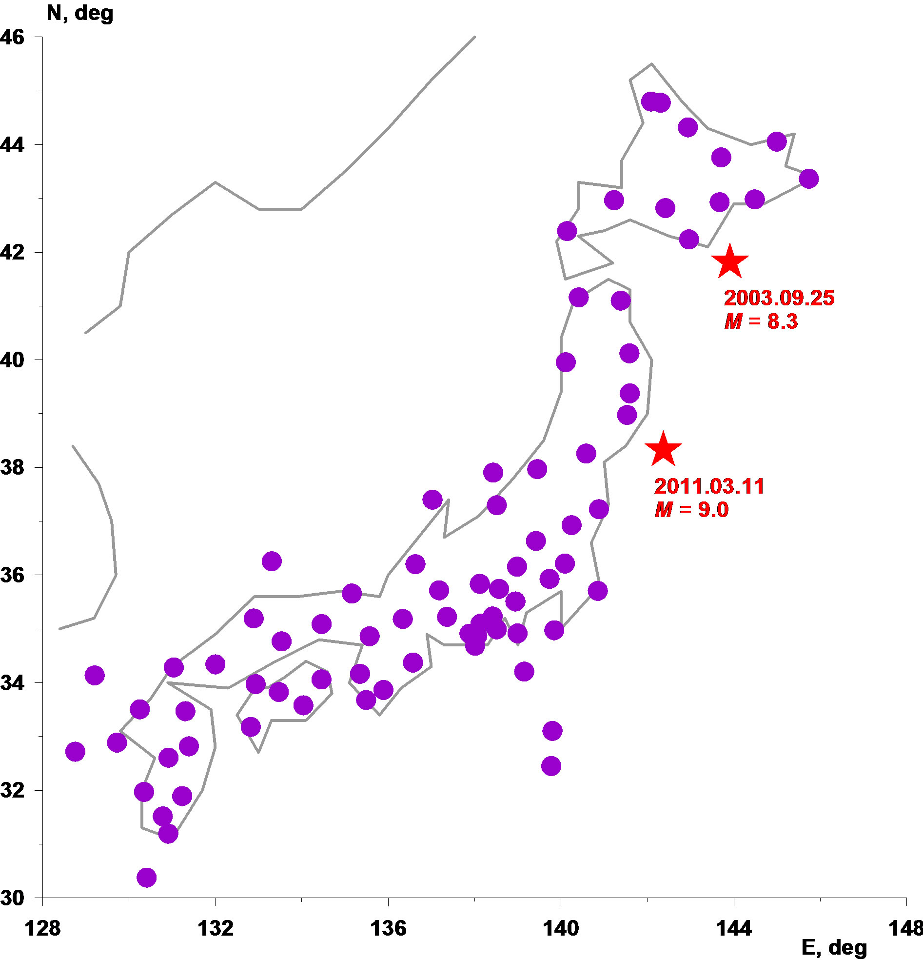
Figure 1. Positions of 77 seismic stations of the network F-net.
noise variations for the analysis equals 2 minutes.
3. THE USED STATISTICS OF SEISMIC NOISE
3.1. Singularity Spectrum Support Width
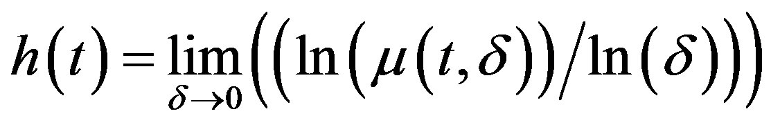
Multifractal singularity spectrum  [17] of the signal
  is defined as a fractal dimensionality of time moments
  which have the same value of local Lipschitz-Holder exponent:
 i.e.
i.e. where
where , maximum and minimum values are taken for argument
 . The value
  is a measure of signal variability in the vicinity of time moment
  [17].
[17].
If  is a usual self-similar monofractal signal with Hurst exponent value
 , then
 but finite sample estimate of singularity spectrum does not obey these rigorous theoretical conditions of course.
Practically the most convenient method for estimating singularity spectrum is a multifractal DFA-method [18] which is used here. The function  could be characterized by following parameters:
and —an argument providing maximum to singularity spectra:
 . Parameter
  could be called a generalized Hurst exponent and it gives the most typical value of Lipschitz-Holder exponent. Parameter
 , singularity spectrum support width, could be regarded as a measure of variety of stochastic behavior. For removing scale-dependent trends (which are mostly caused by tidal variations) in multifractal DFAmethod of singularity spectrums estimates a local polynomials of the 8-th order were used.
3.2. Wavelet-Based Smoothness Index and Minimum Normalized Entropy
The smoothness of the curve usually is defined as the number of its continuous derivatives. But this classic definitions is rather hard to use for applying to random processes. In the paper [9] the notion of integer smoothness index SI was proposed for random signal as the number of vanishing moments of the “best” orthogonal wavelet which is defined for the fragment of the signal from minimum of the value of entropy for distribution of squared wavelet coefficients. We try 17 orthogonal wavelets [19]: 10 usual wavelets of Daubechies (number of vanishing moments equals to integer numbers from 1 up to 10) and 7 a so called symlets with numbers of vanishing moments varying from 4 up to 10. More is the number of vanishing moments more smooth is the orthogonal wavelet and thus, more smooth is the hidden smoothness of random signal.
The by-product of calculating smoothness index is the minimum normalized entropy of squared wavelet coefficients itself. Let  be the finite sample of the signal
 —index, numerating the counts. The normalized entropy is defined by the formula:
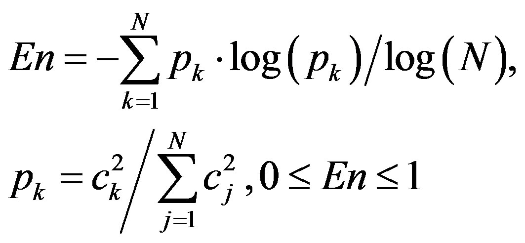 (1)
(1)
Here  are the orthogonal wavelet coefficients which were found from minimized the value (1). For low-frequency noise the parameters
  and
and  were estimated within adjacent time windows of the length
 , i.e. 1 day, after removing trend by polynomial of the 8-th order.
3.3. Index of Linear Predictability
This index was proposed in [9]. Let  be the recorded signal. Let us take “long” adjacent time windows of the length
  counts and consider “short” time window of the length
  counts,
  , which is moving from left to right direction within each “long” adjacent window with minimum mutual shift 1 sample. These “short” time windows are used for constructing two predictors one step ahead within each “long” window.
The 1st predictor is trivial and for each time moment ,
,  , within “long” window, it is calculated as mean value over previous “short” window:
 .
.
Thus, we can compute the error of trivial predictor:  and its variance:
 .
.
The 2nd predictor is based on using correlations between neighbor values of the signal  and use the autoregression model AR(2) of 2nd order:
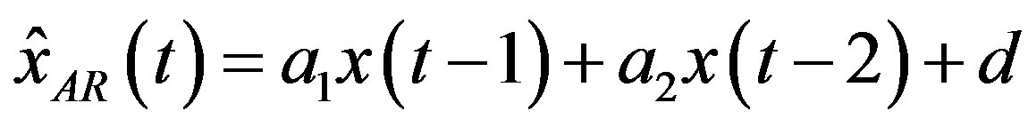 ,
, .
.
Vector of AR(2)-parameters  is defined by least squares method using values of the signal
  within “short” time window of the length
  which is adjacent to time moment
  from left-hand side:
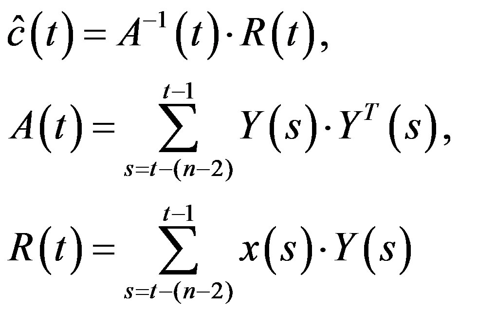 (2)
(2)
where . Similar to trivial predictor we can compute the error of AR(2)-predictor:
 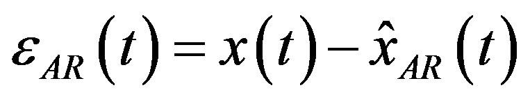 and its variance
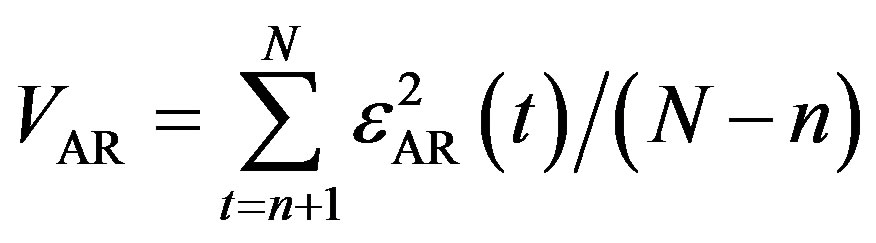 .
.
Index of linear predictability is defined as 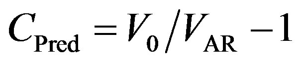 .
.
The 2nd autoregression model AR(2) is selected because this is the minimal order for the AR-model, which enables one to describe the oscillatory motion and could provide the maximum spectral density between the Nyquist frequency and zero [20,21]. The AR-prediction makes use of the correlation property of the nearby values of increments of the recorded signals. If such a correlation exists and signal  is linearly predictable within current “long” time window of the length
  sample then
 , and
, and .
.
For low-frequency noise the linear predictability index was estimated for increments of waveforms. The transition to increments is dictated by the necessity to avoid dominance of low frequencies associated with tides and other trends. In the calculations of the linear predictability index for one-minute data, the estimations were performed in the adjacent long time windows of length , i.e. 1 day. The “short” time window length
 , i.e. 1 hour.
4. RESULTS
The seismic records from each stations after coming to 1 minute sampling time step were split into adjacent time fragments of the length 1 day (1440 samples) and for each fragment parameters ,
,  ,
,  and
and  were calculated. Thus, time series of these 4 values with sampling time step 1 day were obtained from each of 77 seismic stations which are presented at the Figure 1.
Having the values of ,
,  ,
,  and
and  from all seismic stations it is possible to create maps of spatial distribution of these seismic noise statistics. For this purpose let us consider the regular grid of the size 30 × 30 nodes covering the rectangular domain with latitudes between 30˚N and 46˚N and longitudes between 128˚E and 148˚E (see Figure 1). For each node of this grid the daily values of
 ,
,  ,
,  and
and  are corresponded which are calculated as median for the values of five nearest to the node seismic stations. This simple procedure provides the sequence of daily maps of all parameters. The averaged maps are created by averaging daily maps for all days between 2 given dates. Taking into account that almost all stations of the F-net are placed at large Japanese islands these map in the ocean regions have the less significance than at islands of course. But we had to work with those data which we have at our disposal. The method of nearest neighbors which is used in this paper provides a rather natural extrapolation of the used values into domains which have no points of observations.
Figures 2 and 3 present averaged maps of ,
,  ,
,  and
and  for 3 adjacent time fragments: from the beginning of 1997 up to 25 of September 2003, the day of earthquake with magnitude 8.3 near Hokkaido; from 26 of September 2003 up to 10 of March 2011, the day before Tohoku mega-earthquake 11 of March with magnitude 9.0 and from 14 of March 2011 up to 15 of April 2011. Three days, 11, 12 and 13 of March 2011 are excluded from the analysis because during these days a lot of seismic station of F-net were not working properly after seismic shock of 11 of March 2011.
The Figures 2(a') and (b') show that plotting averaged maps of spatial distribution of singularity spectrum support width  could extract the place of future catastrophe as the regions with relatively low values of
 . Figure 2(a') presents a map where the area of relatively low
  could be noticed which includes the place of future mega-earthquake and it is not split into North and South parts. At the Figure 2(b') we can see that after the event 25 of September 2003 this area was split into North and South parts and the North part turned to be the area of aftershocks of Great Japan earthquake of 11 of March 2011 whereas the South part remains to be the region of relatively low values of singularity spectrum support width
  before and after 11 of March 2011 (Figure 2(c')). According to interpretation of regions with low values of
  as the seismically dangerous ones we could propose a hypothesis that during Tohoku earthquake only a half of accumulated seismic energy was dropped and that the above written South region (the north part of Philippine plate, Nankai Through) will be the area of future mega-earthquake with magnitude 8.5 - 9.0. The estimate of magnitude follows from the size of the area of low
  values (Figure 2(c')) which approximately equals to the area of Tohoku earthquake aftershocks.
The Figures 2(a″)-(c″) show that linear predictability index  is a some kind of “antipode” to the parameter
  and almost everything what was written above about properties of
  could be repeated for
  with changing “minimum” to “maximum”: relatively maximum values of linear predictability index extract seismically danger domain before the earthquake.
The Figure 3 presents averaged maps for waveletbased statistics  and
and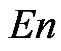 . Smoothness index is defined as integer but after operations of taken median values among 5 nearest to the node stations for mapping it becomes fractional. It could be noticed that these statistics are rather similar to linear predictability index and they are “antipodes” to the parameter
 : they extract the region of future earthquake by their relatively high values. The minimum normalized entropy
  seems even be the most “clean” statistics in comparison with all others: it has no essential maximum values anywhere except the region of Tohoku earthquake and the region of the proposed future earthquake to the south direction from Tokyo. The results presented at the Figures 2 and 3 are remarkable by the fact that 4 statistics which are absolutely different by their construction extract the same regions as seismically danger.
The Figure 4 presents the graphic of daily mean values of smoothness index computed for all stations. This graphic is interesting by the explicit positive trend of seismic noise smoothness which started at the beginning of 2003 and was continuing till the beginning of 2010 when the mean smoothness attains maximum value. After that a time interval of large mean  variability began which include the time moment of Tohoku earthquake and this peculiarity is continuing till now. Maybe when the SI variability became less and mean value became high then it will be a precursor of the next megaearthquake?
5. CONCLUSION AND DISCUSSION
Plotting the maps of different properties of low-frequency seismic noise within moving time window could present a new method of dynamic seismic hazard estimate.
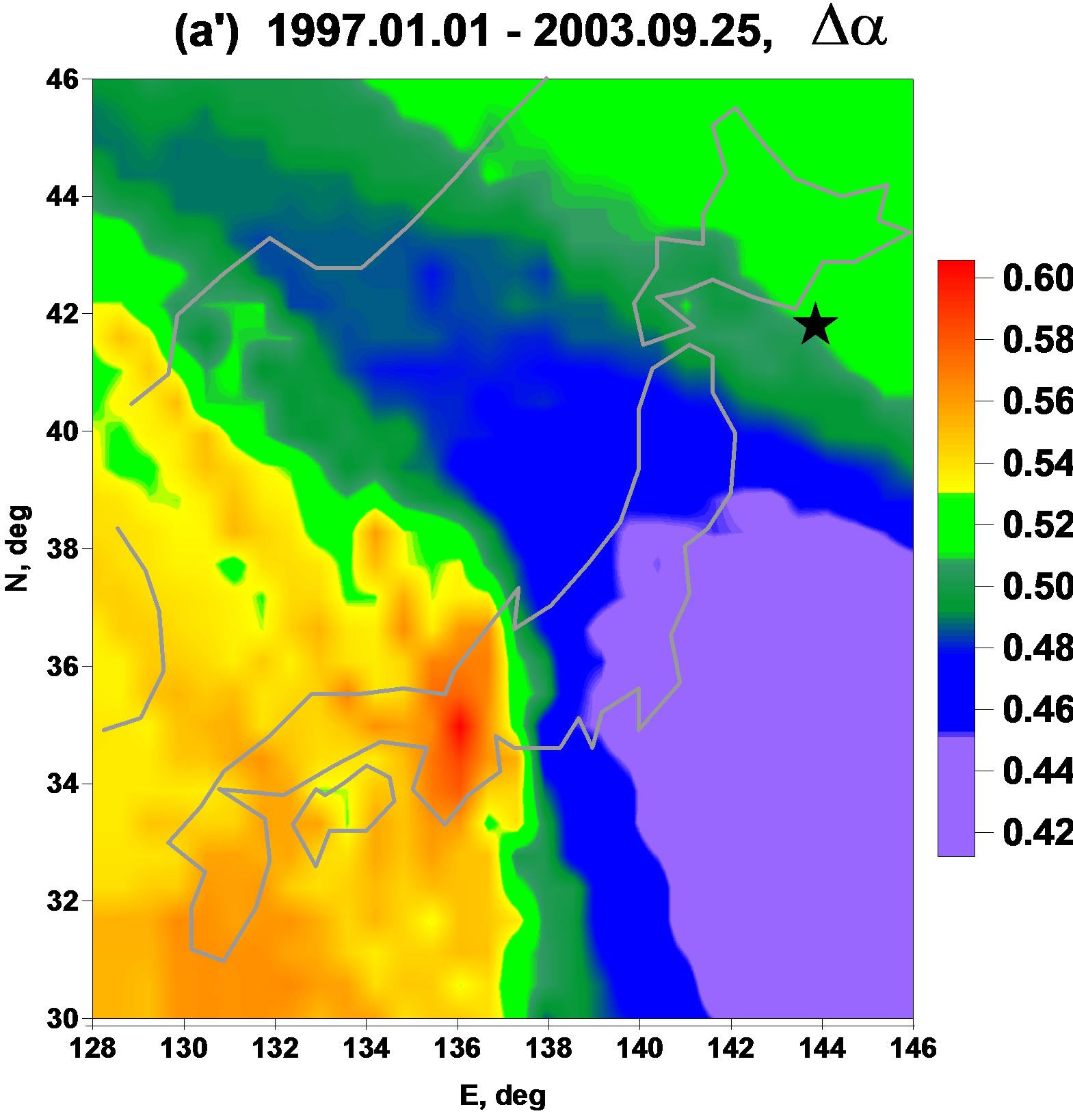
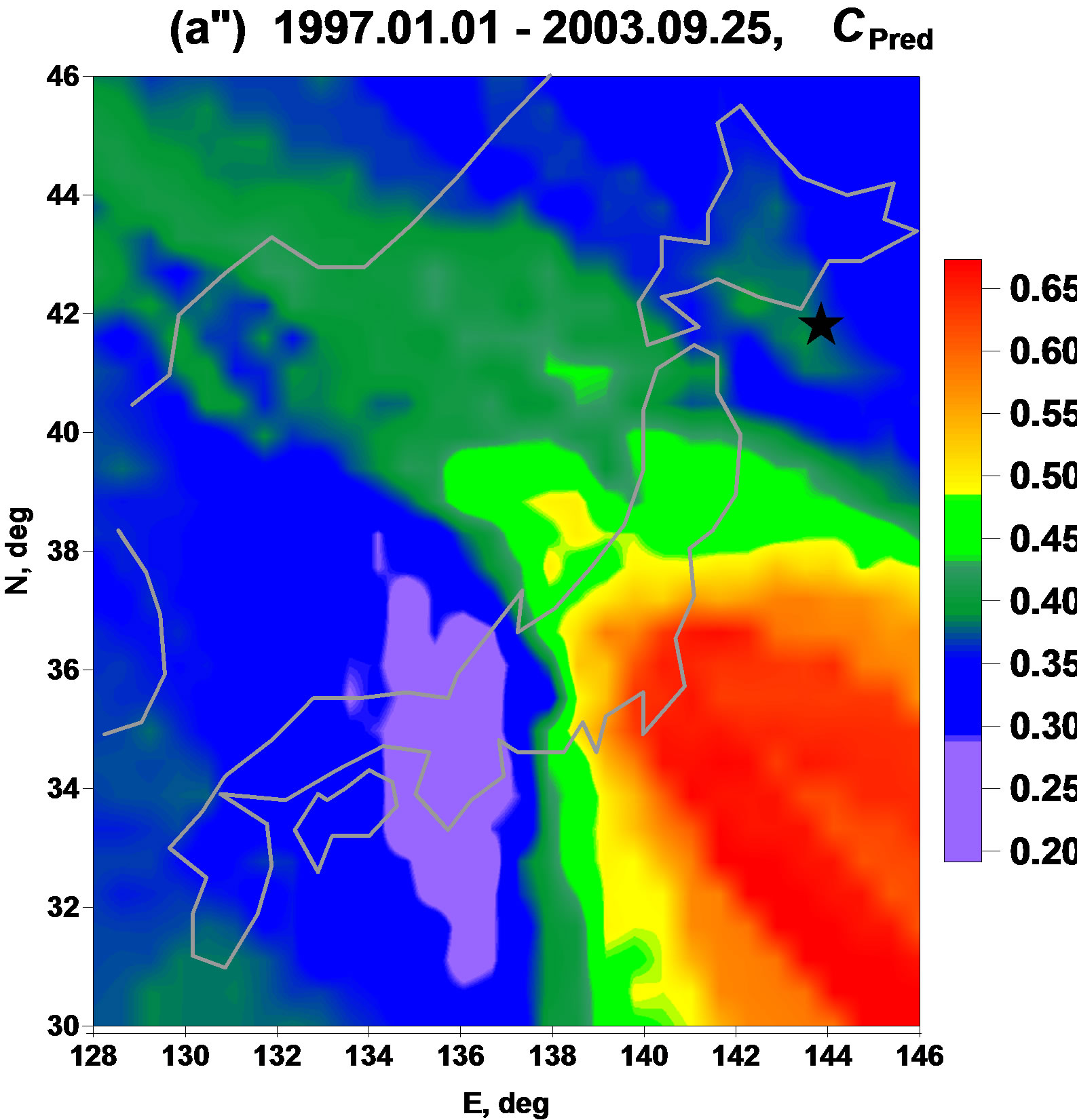
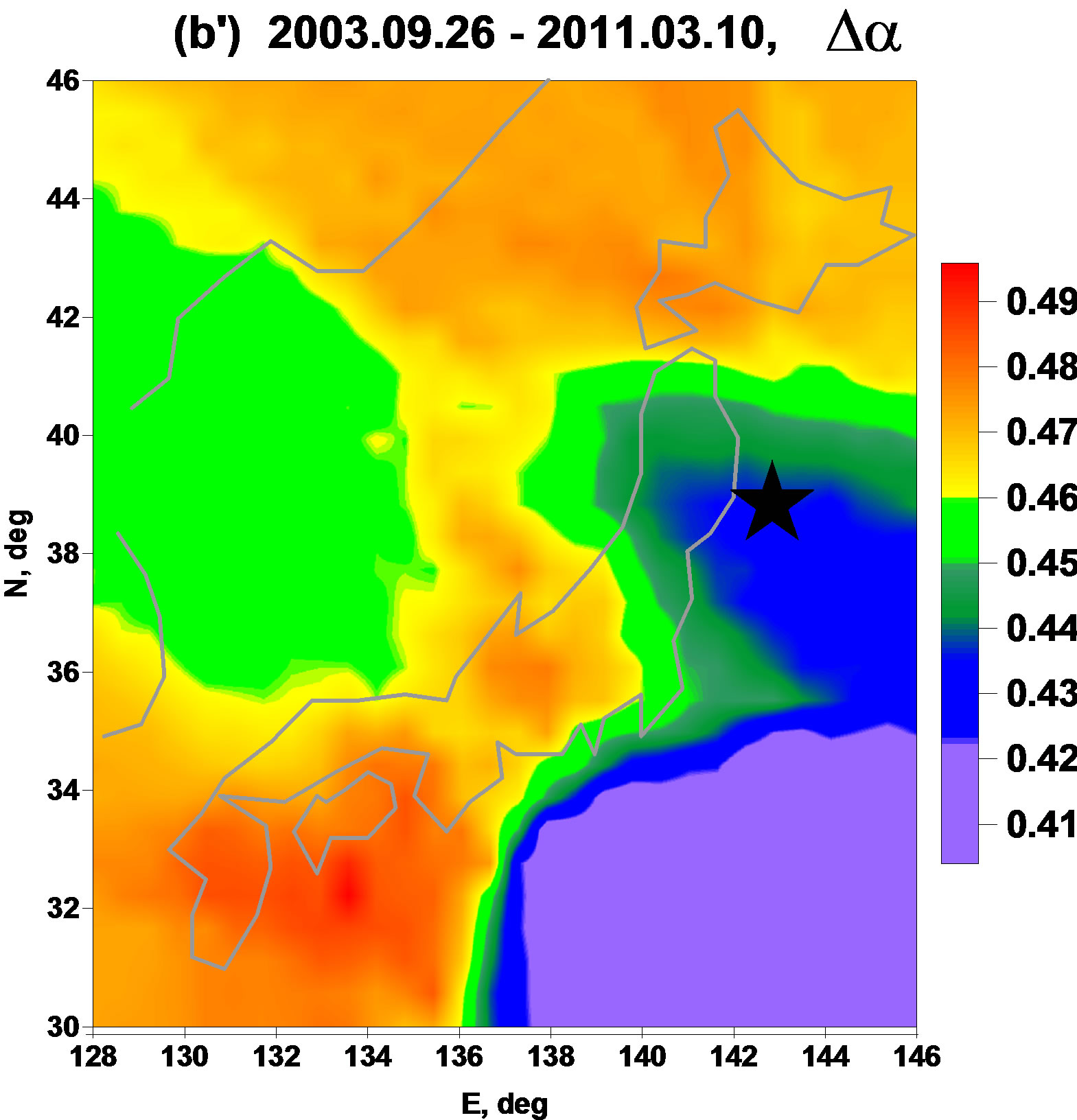
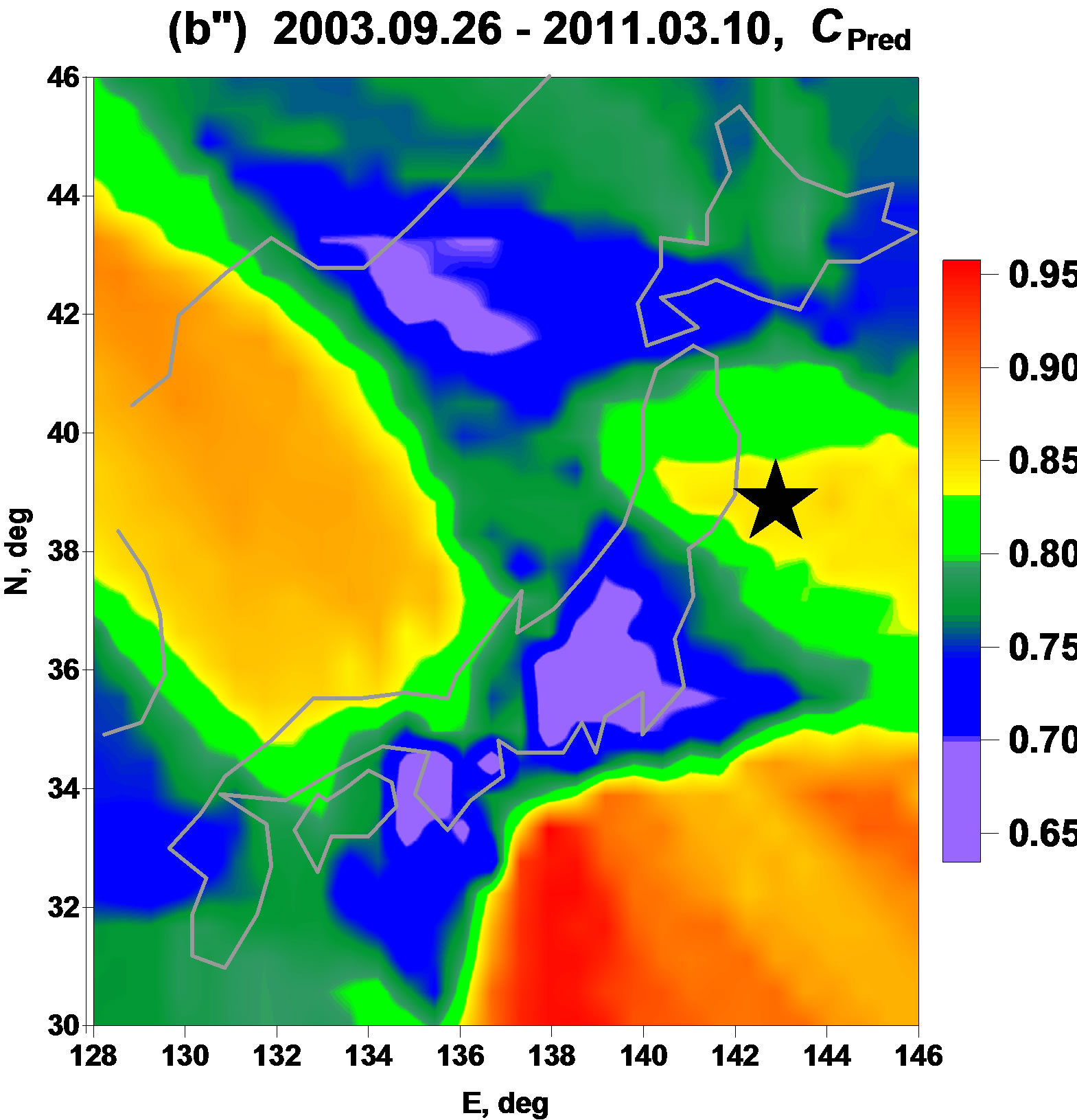
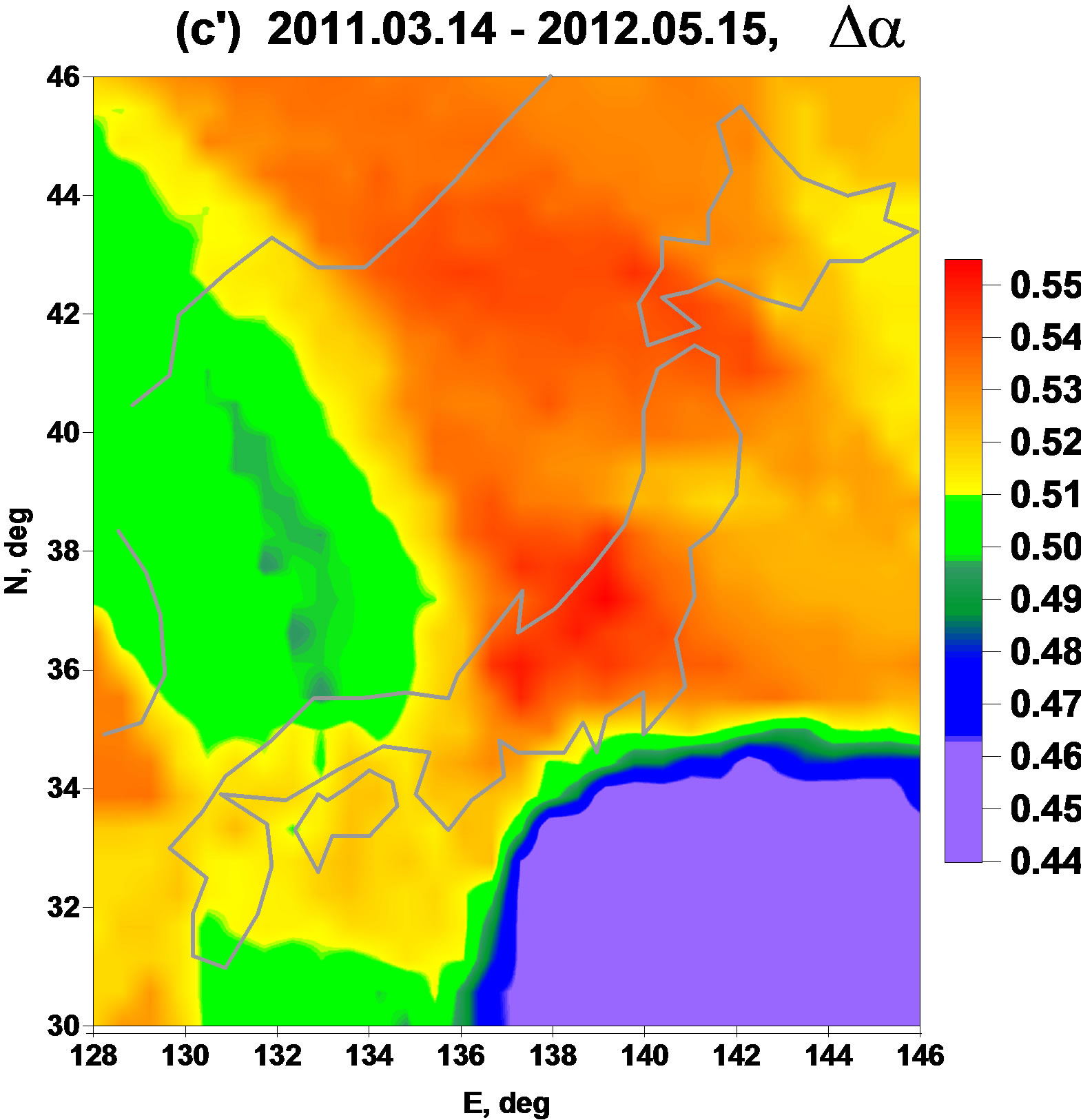
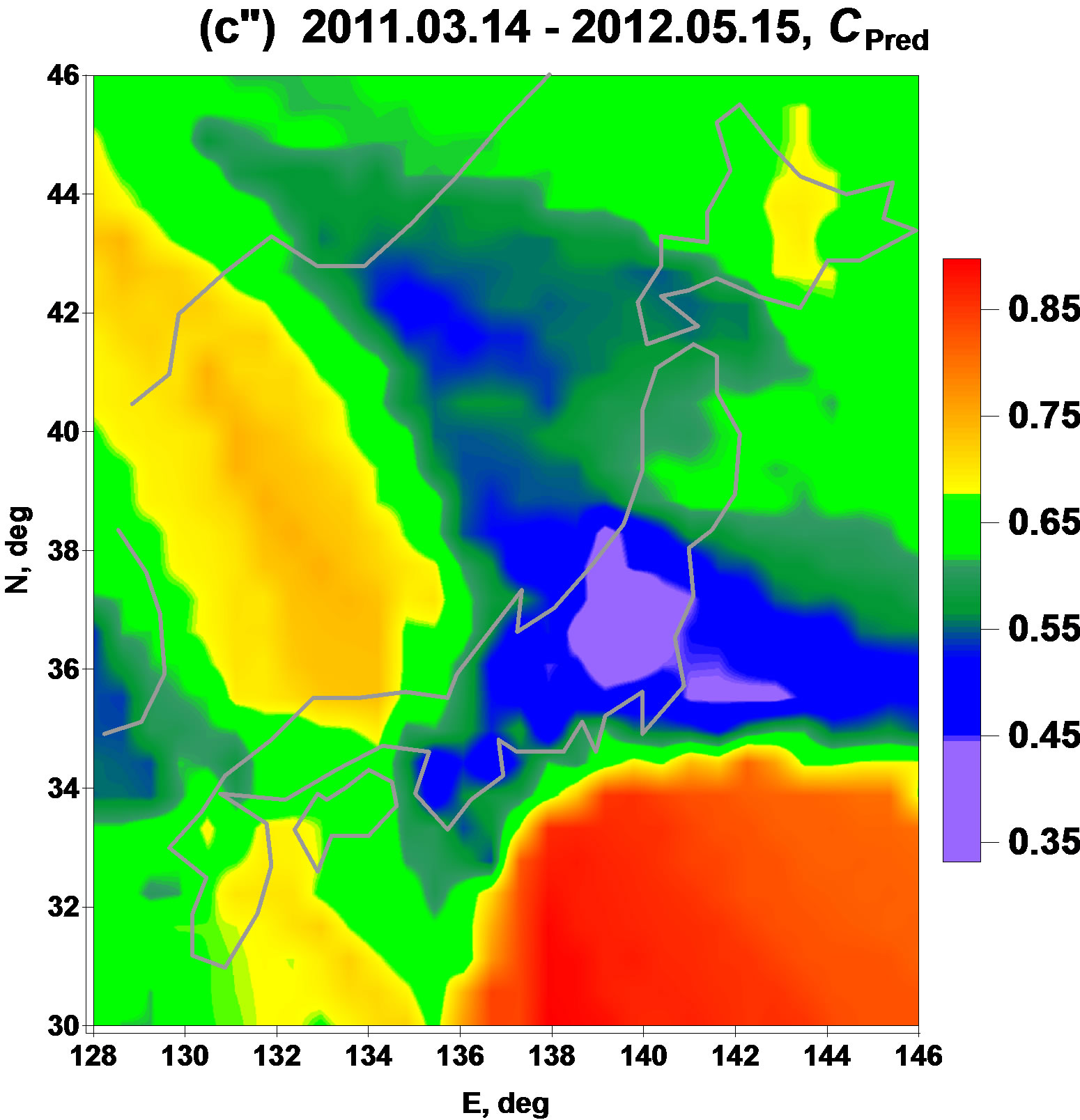
Figure 2. Averaged maps of multi-fractal singularity spectrums support width (a', b', c') and linear predictability index (a″, b″, c″) for 3 successive time intervals. Stars indicate epicenters of earthquakes: 25 of Sept 2003, M = 8.3 (a', a″) and 11 of March 2011, M = 9.0 (b', b″).
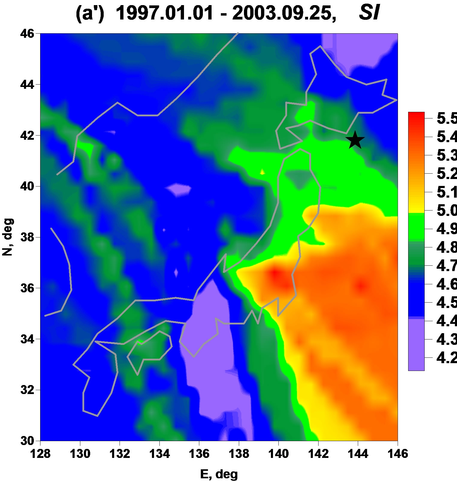
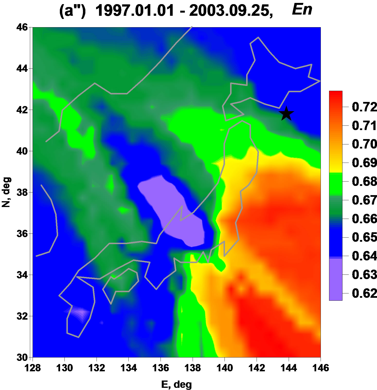
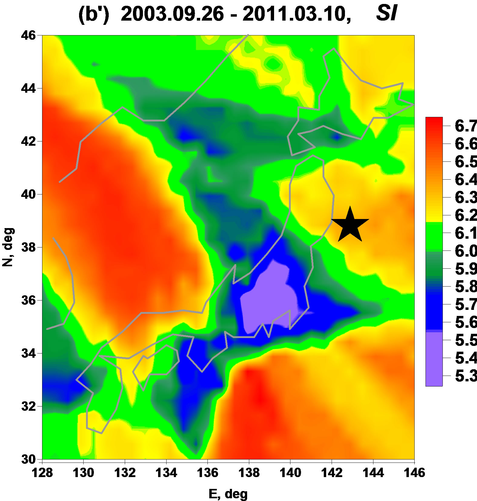
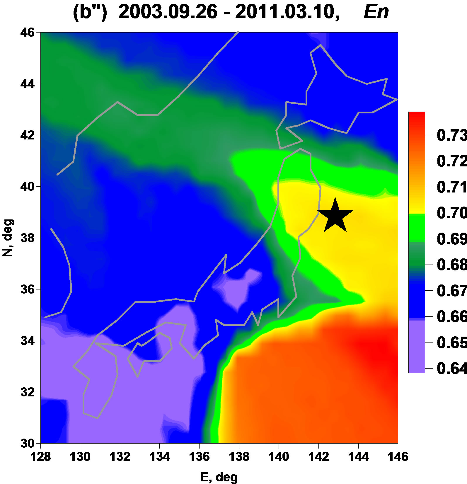
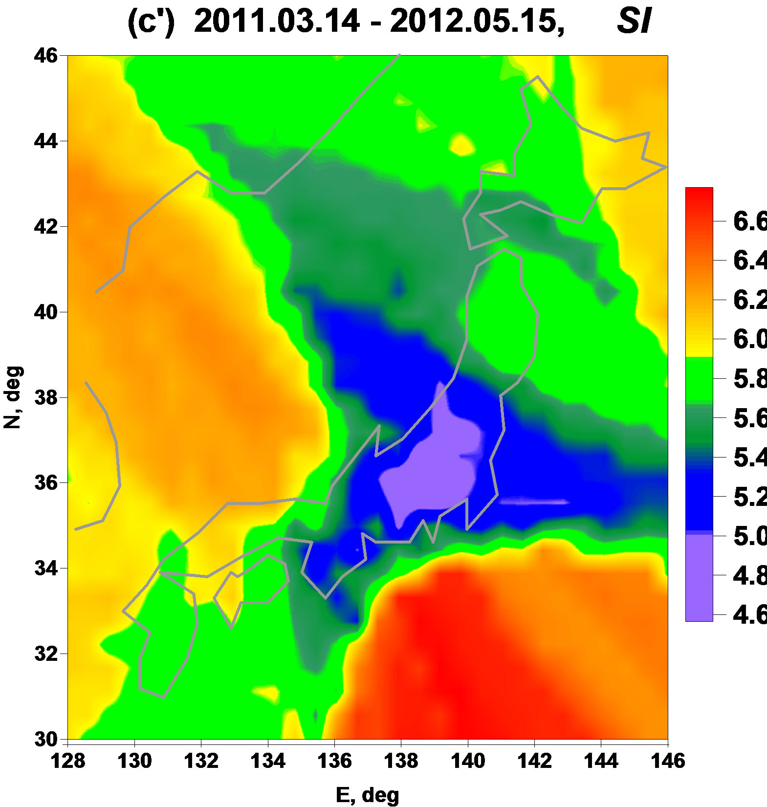
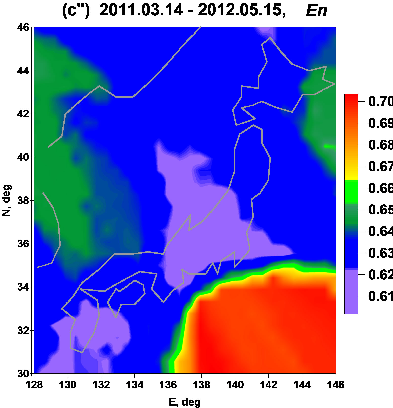
Figure 3. Averaged maps of seismic noise waveforms smoothness index (a', b', c') and minimum normalized entropy of squared wavelet coefficients (a″, b″, c″) for 3 successive time intervals. Stars indicate epicenters of earthquakes: 25 of September 2003, M = 8.3 (a', a″) and 11 of March 2011, M = 9.0 (b', b″).
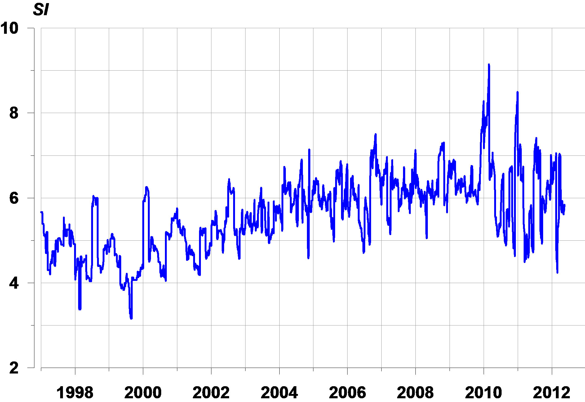
Figure 4. Graphic of daily mean values of seismic noise smoothing index.
It gives a possibility to inspect the origin and evolution of the “spots of danger”. Analysis of seismic noise at Japan islands from broad-band seismic network F-net gave a possibility for prediction of Great Japan earthquake of 11 of March 2011. The prediction was published in a number of scientific papers and abstracts at international conferences in advance of the seismic catastrophe. According to the analysis of seismic noise after 11 of March of 2011 the next mega-earthquake with magnitude 8.5 - 9.0 could occur at the region of Nankai Trough.
Just because the experience of using these statistics is very short it is rather hard now to make an order: which parameters are the most “prognostic” and which are the less ones. After comparing maps at the Figures 2 and 3 it seems that singularity spectrum support width (Figure 2(a')-(c')) and normalized entropy (Figure 3(a″)-(c″)) have “the most strong power” to extract dangerous regions. For more reliable conclusion these methods should be tested in other seismically active regions where a rather dense broad-band seismic networks exist, for instance in California.
The probable physical interpretation of the precursory effects which are presented at this paper could be the following. Hierarchical self-similar block structure of the Earth’s crust [22,23] has a consequence of existence of a lot of blocks with different sized (scales) which are at different stages of their consolidation from their constitutive parts (block of less sizes). In dependence on the state of consolidation and on the range of the block within Earth’s crust structure hierarchy the transfer and resonance properties of the block are different. A great variety of consolidated block sizes follows a large multifractal singularity spectrum support width of low-frequency seismic noise which is generated as a result of seismic waves propagation from atmosphere and oceanic sources through hierarchical block medium consisting of blocks with different transfer and resonance properties.
Seismic noise is a multifractal random process because the hierarchical medium (consisting of consolidated blocks of different ranges) of seismic waves propagation is multifractal. What happens before the strong earthquake? In order that strong earthquake could occur it is necessary the existence of a consolidated crust block of large size—otherwise the energy could not be accumulated and will be dissipated in a large number of small earthquakes. The existence of the large consolidated block of Earth’s crust means the loss of variety of transfer and resonance properties of the medium (it becomes more uniform). The loss of variety of medium properties follows the loss of multifractality, i.e. the decreasing of . Thus, if the mean value of
  is decreasing it is an indicator of consolidation of large block of the Earth’s crust and increasing of seismic danger.
The consolidation of small blocks into the large one before the strong earthquake has a consequence that mutual movements of small blocks canceled. It means that the low-frequency seismic noise does not include now high amplitude variations which are connected with these mutual movements. The absence of high amplitude variations (“low-frequency spikes”) follows the high value of entropy of squared wavelet coefficients distribution. For the same reason the noise became more smooth and more predictable.
6. ACKNOWLEDGEMENTS
This work was supported by the Russian Foundation for Basic Research (project no. 12-05-00146) and Russian Ministry of Science (project no. 11.519.11.5024). The author is grateful to National Institute for Earth Science and Disaster Prevention (NIED), Japan, for providing free access to the source of broadband seismic noise waveforms registered at the F-net stations.
REFERENCES
- Kobayashi, N. and Nishida, K. (1998) Continuous excitation of planetary free oscillations by atmospheric disturbances. Nature, 395, 357-360. doi:10.1038/26427
- Tanimoto, T. (2001) Continuous free oscillations: atmosphere-solid Earth coupling. Earth and Planetary Sciences, 29, 563-584. doi:10.1146/annurev.earth.29.1.563
- Tanimoto, T. (2005) The oceanic excitation hypothesis for the continuous oscillations of the Earth. Geophysical Journal International, 160, 276-288. doi:10.1111/j.1365-246X.2004.02484.x
- Rhie, J. and Romanowicz, B. (2004) Excitation of Earth’s continuous free oscillations by atmosphere-ocean-seafloor coupling. Nature, 431, 552-554. doi:10.1038/nature02942
- Lyubushin, A.A. (2008) Multifractal properties of lowfrequency microseismic noise in Japan, 1997-2008. Book of abstracts of 7th General Assembly of the Asian Seismological Commission and Japan Seismological Society, 2008 Fall meeting, Tsukuba, 24-27 November 2008, 92.
- Lyubushin, A.A. (2009) Synchronization trends and rhythms of multifractal parameters of the field of low-frequency microseisms. Izvestiya Physics of the Solid Earth, 45, 381-394. doi:10.1134/S1069351309050024
- Lyubushin, A.A. (2010) Synchronization of multifractal parameters of regional and global low-frequency microseisms. European Geosciences Union General Assembly, Vienna, 2-7 May 2010, 696.
- Lyubushin, A.A. (2010) Synchronization phenomena of low-frequency microseisms. European Seismological Commission: 32nd General Assembly, 6-10 September 2010, Montpelier, 124.
- Lyubushin, A.A. (2010) The statistics of the time segments of low-frequency microseisms: trends and synchronization. Izvestiya Physics of the Solid Earth, 46, 544-554. doi:10.1134/S1069351310060091
- Lyubushin, A.A. (2010) Multifractal parameters of lowfrequency microseisms. In: V. de Rubeis et al., Eds., Synchronization and triggering: from fracture to earthquake processes, Springer-Verlag, Berlin Heidelberg.
- Lyubushin, A.A. (2011) Cluster analysis of low-frequency microseismic noise. Izvestiya Physics of the Solid Earth, 47, 488-495. doi:10.1134/S1069351311040057
- Lyubushin, A.A. (2011) Seismic catastrophe in Japan on March 11, 2011: long-term prediction on the basis of lowfrequency microseisms. Izvestiya Atmospheric and Oceanic Physics, 46, 904-921. doi:10.1134/S0001433811080056
- Lyubushin, A.A. (2011) Prediction of Tohoku seismic catastrophe by microseismic noise multi-fractal properties. Abstract S53A-2273 presented at 2011 Fall Meeting, American Geophysical Union, San Francisco, 5-9 December 2011.
- Ivanov, P.Ch., Amaral, L.A.N., Goldberger, A.L., Havlin, S., Rosenblum, M.B., Struzik, Z. and Stanley, H.E. (1999) Multifractality in healthy heartbeat dynamics. Nature, 399, 461-465. doi:10.1038/20924
- Pavlov, A.N. and Anishchenko, V.S. (2007) Multifractal analysis of complex signals. Physics-Uspekhi, 50, 819-834. doi:10.1070/PU2007v050n08ABEH006116
- Humeaua, A., Chapeau-Blondeau, F., Rousseau, D., Rousseau, P., Trzepizur, W. and Abraham, P. (2008) Multifractality, sample entropy, and wavelet analyses for age-related changes in the peripheral cardiovascular system: Preliminary results. Medical Physics, 35, 717-727. doi:10.1118/1.2831909
- Feder, J. (1988) Fractals. Plenum Press, New York.
- Kantelhardt, J.W., Zschiegner, S.A., Konscienly-Bunde, E., Havlin, S., Bunde, A. and Stanley, H.E. (2002) Multifractal detrended fluctuation analysis of nonstationary time series. Physica A: Statistical Mechanics and Its Applications, 316, 87-114. doi:10.1016/S0378-4371(02)01383-3
- Mallat, S. (1998) A wavelet tour of signal processing. Academic Press, San Diego.
- Box, G.E.P. and Jenkins, G.M. (1970) Time series analysis: Forecasting and control. Holden-Day. San Francisco.
- Kashyap, R.L. and Rao, A.R. (1976) Dynamic stochastic models from empirical data. Academic Press, New York.
- Hirata, T., Satoh, T. and Ito, K. (1987) Fractal structure of spatial distribution of microfacturing in rock. Geophysical Journal of the Royal Astronomical Society, 90, 369-377. doi:10.1111/j.1365-246X.1987.tb00732.x
- Turcotte, D.L. (1997) Fractals and chaos in geology and geophysics. 2nd edition, Cambridge University Press, New York. doi:10.1017/CBO9781139174695