Engineering
Vol.5 No.5(2013), Article ID:31701,7 pages DOI:10.4236/eng.2013.55063
Runge-Kutta Schemes Coefficients Simulation for Comparison and Visual Effects
Department of Mechanical Engineering, University of Ibadan, Ibadan, Nigeria
Email: ooe.ajide@mail.ui.edu.ng
Copyright © 2013 Salau Tajudeen Abiola Ogunniyi, Ajide Olusegun Olufemi. This is an open access article distributed under the Creative Commons Attribution License, which permits unrestricted use, distribution, and reproduction in any medium, provided the original work is properly cited.
Received January 25, 2013; revised March 26, 2013; accepted April 3, 2013
Keywords: Runge-Kutta; Visual Effects; Simulation Coefficients; Taylor Series and Butcher Assumptions
ABSTRACT
Runge-Kutta scheme is one of the versatile numerical tools for the simulation of engineering systems. Despite its wide and acceptable engineering use, there is dearth of relevant literature bordering on visual impression possibility among different schemes coefficients which is the strong motivation for the present investigation of the third and fourth order schemes. The present study capitalise on results of tedious computation involving Taylor series expansion equivalent supplemented with Butcher assumptions and constraint equations of well-known works which captures the essential relationship between the coefficients. The simulation proceeds from random but valid specification of two out of the total coefficients possible per scheme. However the remaining coefficients are evaluated with application of appropriate function relationship. Eight and thirteen unknown coefficients were simulated respectively for third and fourth schemes over a total of five thousand cases each for relevant distribution statistics and scatter plots analysis for the purpose of scheme comparison and visual import. The respective three and four coefficients of the slope estimate for the third and fourth schemes have mix sign for large number of simulated cases. However, none of the two schemes have above three of these coefficients lesser than zero. The percentages of simulation results with two coefficients lesser than zero dominate and are respectively 56.88 and 77.10 for third and fourth schemes. It was observed that both popular third and fourth schemes belong to none of the coefficients being zero classification with respective percentage of 0.72 and 3.28 in total simulated cases. The comparisons of corresponding scatter plots are visually exciting. The overall difference between corresponding scatter plots and distribution results can be used to justify the accuracy of fourth scheme over its counterpart third scheme.
1. Introduction
The versatility of Runge-Kutta scheme as a numerical tool in engineering (most especially nonlinear dynamics) is well acknowledged among researchers in this field. [1] has employed Runge-Kutta scheme in modelling Lorenz system. In the authors’ paper, the classical fourth-order Runge-Kutta was modified to obtain new methods which are of order five. These techniques were tested on the Lorenz system involving chaotic and nonchaotic characteristics. The results obtained shows that Lorenz model is highly sensitive to the initial conditions of the system. The paper concluded that modified fifth-order RungeKutta method appears to be the best method to approximate Rayleigh-Benard convection. This is attributed to its high accuracy. [2] has also demonstrated the versatility of the Runge-Kutta scheme. In their paper, an em-
bedded Runge-Kutta with orders 3 and 4 with the aim to deliver an estimation of the local error for adaptive stepsize control purposes in the interaction picture method. The results of their study showed that the embedded Runge-Kutta method 4(3) with interaction picture preserves the features of the RK4-IP method and provides a local error estimate at no significant cost. The outcome of their study is of immense advantage in step-size control in the interaction picture method. A recent developed Runge-Kutta scheme has been applied in non-slip rolling [3]. This method is referred to as Accelerated RungeKutta Methods (ARM). This method benefits from precise parameter selection technique that increases their order of accuracy for some problems. The paper showed that an efficient and effective Accelerated Runge-Kutta Method capable of modelling complex nonlinear mechanical systems has been developed. A parametric study of nonlinear beam vibration resting on linear elastic foundation was carried out by [4]. A well known Duffing oscillator was analyzed numerically using Runge-Kutta scheme. The result of the study shows that the stretching potential energy was responsible for generating the cubic nonlinearity in the system dynamic. A low-dispersion and low-dissipation implicit Runge-Kutta has been introduced by [5]. This new implicit Runge-Kutta scheme is of great advantage because high order accuracy is achieved with fewer stages when compared to the standard explicit Runge-Kutta schemes. This method has high application potentials in wall-bounded flows with solid boundaries in the computation as well as sound generation by reacting flows. Visual tools have in no small measure contributed immensely in exploring dynamics of nonlinear systems. [6] carried out a study on the visual effects of filtered chaotic signals. It was understood from the paper that filtered chaotic signals is capable of exhibiting an increase in observed fractal dimension. The approach towards providing an interesting insight into this dynamic is through the use of computer animation and three-dimensional ray-tracings. [7] in his paper reported how fuzzy dynamic system can illustrate chaotic phenomena and chaotic dynamics in comparison to other nonlinear systems. It is concluded from the paper that fuzzy chaotic dynamic model of a cubic map results in the same (visual effects) as bifurcation diagrams, and that it reveals stable equilibrium points, periodic-doubling and chaotic attractors. This study has extensively justified the numerous benefits of visual effects. The possibilities for describing sitting postural control using nonlinear method have been investigated by [8] during a long-term driving. The results obtained show that contrary to conventional analysis procedures, nonlinear measures demonstrated the capability of identifying a threshold behaviour describing the change in discomfort. The visual recurrence plots showed an outstanding change in the underlying dynamics after one hour of driving. [9] explained that the challenge of many other methods used for analyzing chaotic systems was that they depicts local nature and exhibited only limited information about a group of parameters. This challenge motivated these authors in exploring visualization technique on the basis of Mandelbrot set methodology. This help immensely in giving the overall view of chaotic systems dynamic performance in the parameter space. A periodic parametric perturbation has been designed for controlling and chaotification from a three-dimensional autonomous system [10]. Lyapunov exponents and bifurcation diagram were used as visual aids for explaining the abundant dynamic characteristics of a three-dimensional system. The authors’ paper has shown that when there is a small parametric perturbation, highly unique dynamic system behaviour will be experienced. A 4-dimensional Chua system has been characterized by [11] using Lyapunov exponent diagrams. With the introduction of a feedback controller into the system, both the largest and the second largest Lyapunov exponents were considered in Lyapunov exponent diagrams. [12] reported that in exploring the nonlinear dynamics of a periodically Driven Duffing resonator coupled to a Van der pol oscillator, bifurcation diagram was adopted as the visual aids. The behaviour of the coupled system as well as the dependence of the system dynamics on the parameter have been studied using bifurcation analysis. [13] focused on simulation and visualisation of chaotic systems. The study implemented fundamental algorithms from the field of chaotic system dynamics such as the reconstruction of the system trajectory in the appropriate embedding space, and the estimation of Lyapunov exponents and the fractal dimension. The bifurcation diagrams produced provides a significant visual effect for identifying chaotic regions in the parameter space.
Although the available literature on the use of RungeKutta scheme for engineering applications is inexhaustible; the dearth of relevant literature bordering on visual impression possibility among different schemes coefficients is a subject of concern. This strongly motivated the present study of the third and fourth order schemes.
2. Methodology
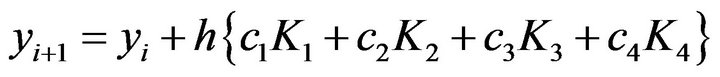
[14] refers, the numerical method of Runge-Kutta is devoted to solving ordinary differential equations of the general form given by Equation (1). However the step by step numerical solution of Equation (1) is given by Equation (2), with ![]() being an incremental weighting function. The general form for
being an incremental weighting function. The general form for ![]() is given by Equation (3). According to Equation (3), the slope estimate of
is given by Equation (3). According to Equation (3), the slope estimate of ![]() is used to extrapolate from an old value
is used to extrapolate from an old value  to a new value
  over a step size h.
 (1)
(1)
 (2)
(2)
 (3)
(3)
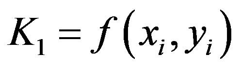
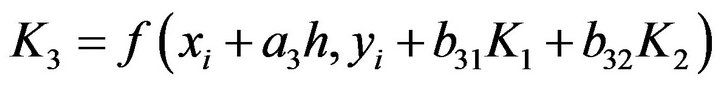
The functions  to
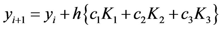
to  for the third and fourth order Runge-Kutta schemes are given by Equations (4) to (7). However, the equivalent of Equation (2) for the third and fourth schemes is given respectively by (8) and (9).
 (4)
(4)
 (5)
(5)
 (6)
(6)
 (7)
(7)
 (8)
(8)
 (9)
(9)
[15] executed the tedious computation of the unknown constant coefficients in Equations (4) to (9) using the equivalent relationship with the corresponding coefficients in Taylor series expansion of the function  to the nth-order terms. The computation was aided by Butcher simplifying assumption implied by Equation (10).
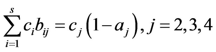 (10)
(10)
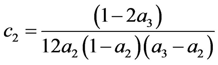
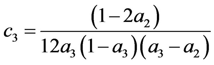
As such the coefficients definitions for the third and fourth order schemes are (11) to (16) and (18) to (28) respectively subject to arbitrary choices of  and
and .
.
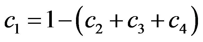
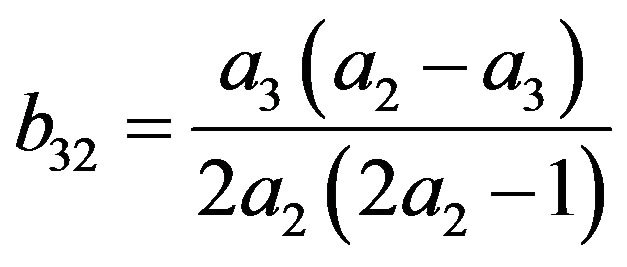
2.1. Third Order Scheme
 (11)
(11)
 (12)
(12)
 (13)
(13)
 (14)
(14)
 (15)
(15)
 (16)
(16)
The constraint conditions for Equations (11) to (16) are detailed in Equation (17).
 (17)
(17)
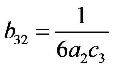
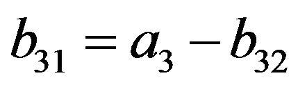
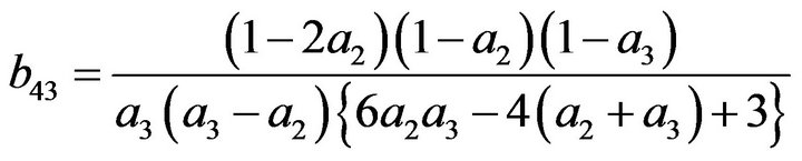
2.2. Fourth Order Scheme
 (18)
(18)
 (19)
(19)
 (20)
(20)
 (21)
(21)
 (22)
(22)
 (23)
(23)
 (24)
(24)
 (25)
(25)
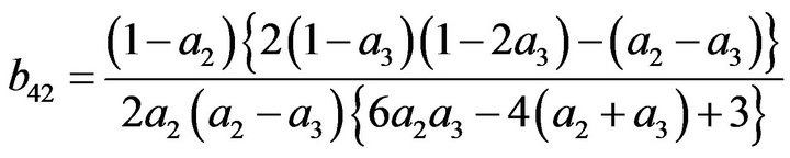 (26)
(26)
 (27)
(27)
 (28)
(28)
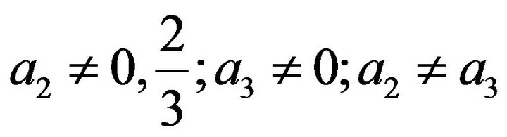
The constraint conditions for Equations (18) to (28) are detailed in Equations (29) and (30).
 (29)
(29)
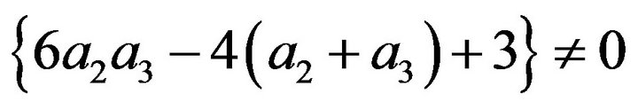 (30)
(30)
2.3. Simulation Parameters
The simulation parameters included arbitrarily selected random number generation seed value of 9876 which drives the random selection of 5000 distinct combination of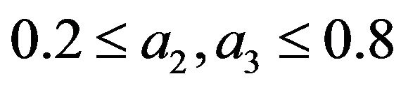 . The success criterion for a trial is that the absolute value of all the coefficients be less or equal to 5.0.
3. Results and Discussions
The simulation results were obtained using FORTRAN 90 while the graphical package is Microsoft Excel 2003. The sample results for the third and fourth order RungeKutta scheme are shown in Tables 1 and 2.
Tables 1 and 2 refers. It is observed that at least one of the coefficients (![]() to
to ) require in Equation (8) is less than zero. Similarly, at least one of the coefficients (
![]() to
to ) require in Equation (9) is also less than zero. However Table 3 shows that none of the two schemes have above three of these coefficients lesser than zero. The percentage of simulation results with two coefficients lesser than zero are respectively 56.88 and 77.10 for third and fourth order schemes. It is interesting to note that both popular third and fourth order RungeKutta schemes belong to none of the coefficients being zero classification.
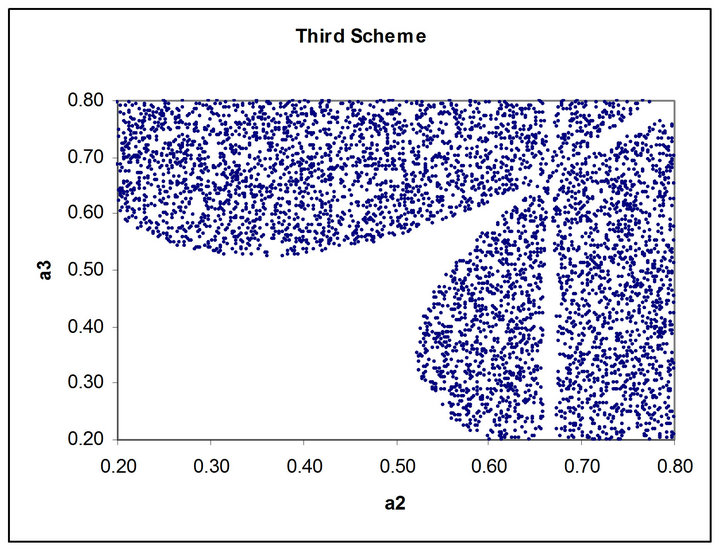
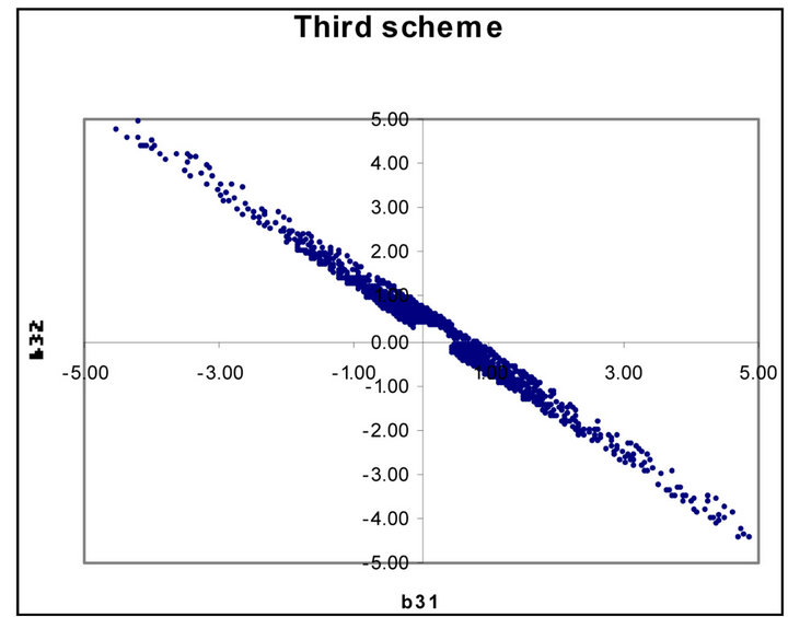
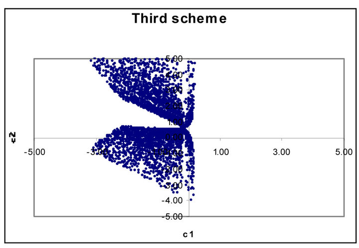
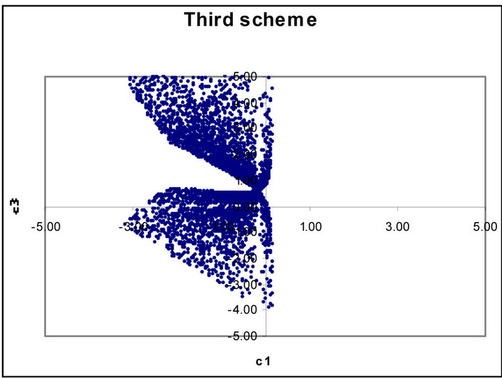
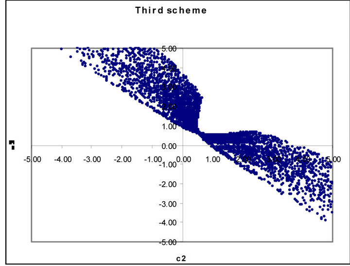
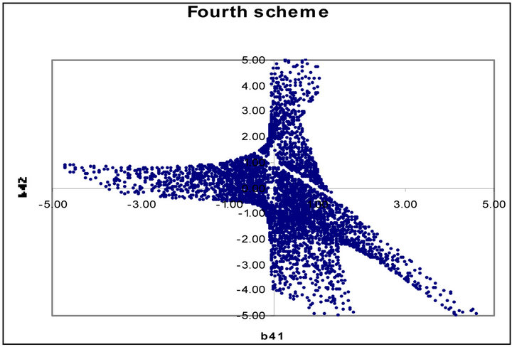
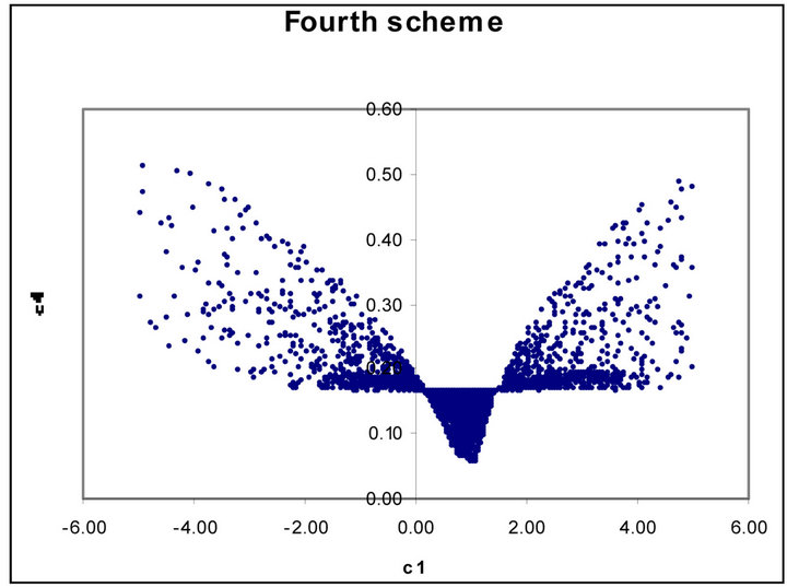
Figures 1 to 5 show dramatic visual differences between corresponding scatter plots with the exception only in Figure 2 in which the plots almost agreed perfectly. Figures 3 and 4 look visually identical. The visual appearance of Figures 6(a) to (c) resemble distorted saddle which is a manifestation of nonlinear dependence of b41, b42 and b43 on a2, a3 and a4 as independent variables

Table 1. Selected simulation results for the third order scheme.
(see Equations (26)-(28)) while there is no corresponding figures for the third order scheme. Similarly Figures 7(b) and (c) look identical to each other while Figure 7(a) is a plane mirror image of Figure 7(b). The region of valid coefficients pair combination is very small compared to total available space region for all the plots in Figures 1 to 7. Despite this space bound constraint majority of the plots are noted for their visual excitement. The observed visual differences in these plots can be a good explanation for the noted computation accuracy potential of fourth scheme over its counterpart third order scheme.
4. Conclusion
This study have shown that the coefficients of the slope estimate for the third and fourth schemes have mix sign for large number of simulated cases. However, none of
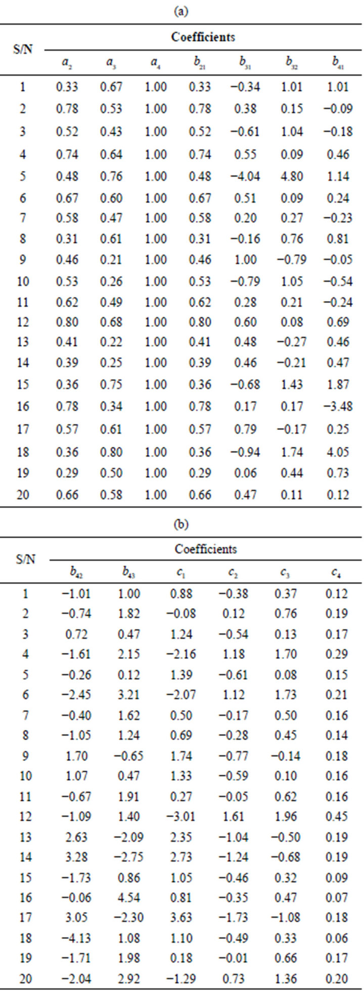
Table 2. Selected simulation results for the fourth order scheme.
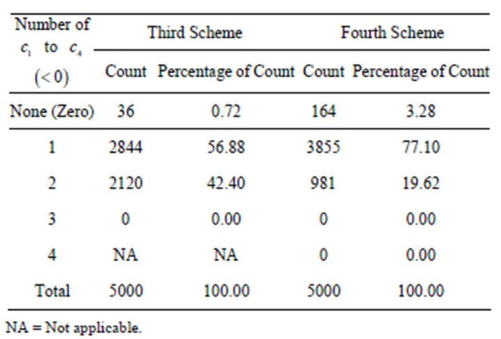
Table 3. Distribution statistic of 5000 simulated (![]() to
to ) and (
![]() to
to![]() ).
).
 (a)
(a)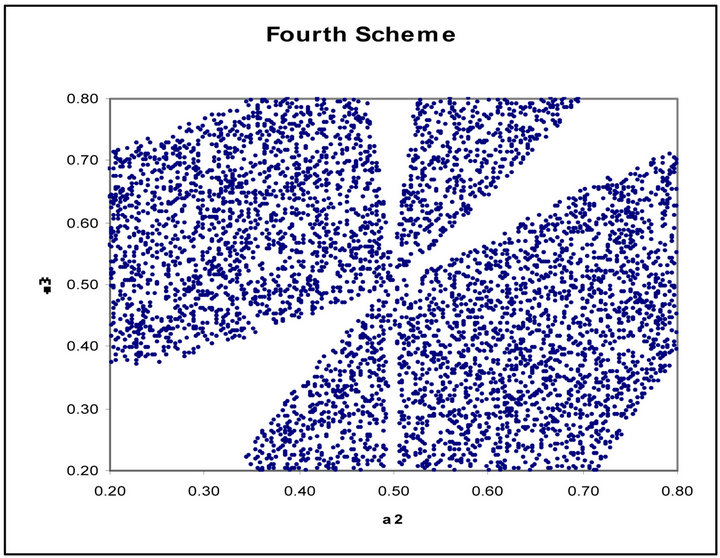 (b)
(b)
Figure 1. (a) Scatter plot of valid  versus
  for third order Runge-Kutta; (b) Fourth order Runge-Kutta.
the two schemes have above three of these coefficients lesser than zero. The percentages of simulation results with two coefficients lesser than zero dominate and are
 (a)
(a)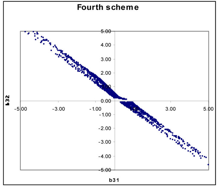 (b)
(b)
Figure 2. (a) Scatter plot of valid  versus
  for third order Runge-Kutta schemes; (b) Fourth order Runge-Kutta schemes.
 (a)
(a)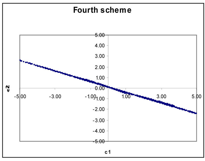 (b)
(b)
Figure 3. (a) Scatter plot of valid ![]() versus
versus  for third order Runge-Kutta schemes; (b) Fourth order Runge-Kutta schemes.
 (a)
(a) (b)
(b)
Figure 4. (a) Scatter plot of valid ![]() versus
versus  for third order Runge-Kutta schemes; (b) Fourth order RungeKutta schemes
 (a)
(a)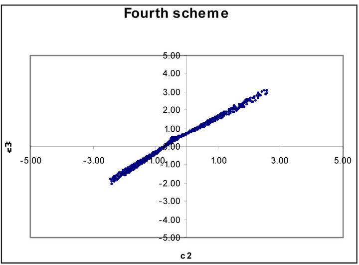 (b)
(b)
Figure 5. (a) Scatter plot of valid  versus
  for third order Runge-Kutta schemes; (b) Fourth order Runge-Kutta schemes.
 (a)
(a) (b)
(b)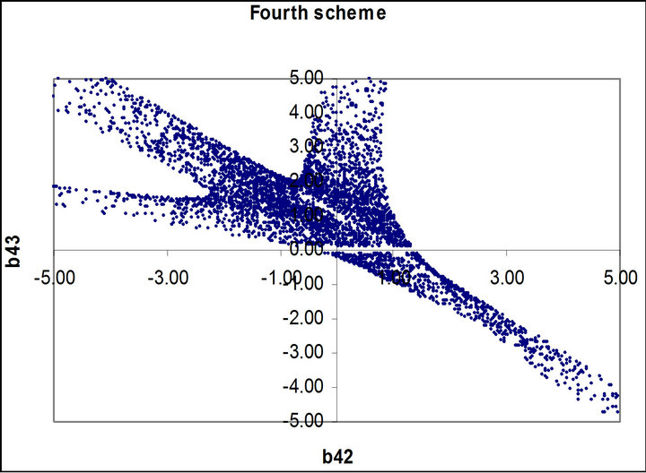 (c)
(c)
Figure 6. (a) Scatter plot of valid 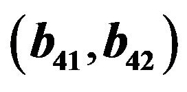 for the fourth order Runge-Kutta scheme; (b) Scatter plot of valid
 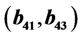 for the fourth order Runge-Kutta scheme; (c) Scatter plot of valid
  for the fourth order RungeKutta scheme.
respectively 56.88 and 77.10 for third and fourth schemes. The popular third and fourth schemes belong to none of the coefficients being zero classification with respective percentage of 0.72 and 3.28 in total simulated cases. The comparisons of corresponding scatter plots are visually exciting. The noted overall visual differences between corresponding scatter plots and distribution results
 (a)
(a)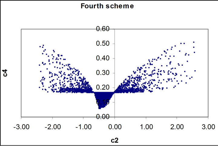 (b)
(b)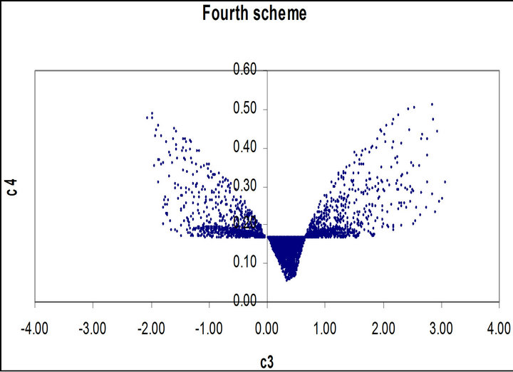 (c)
(c)
Figure 7. (a) Scatter plot of valid  for the fourth order Runge-Kutta scheme; (b) Scatter plot of valid
  for the fourth order Runge-Kutta scheme; (c) Scatter plot of valid
  for the fourth order RungeKutta scheme.
can be used to justify the accuracy of fourth scheme over its counterpart third scheme.
REFERENCES
- R. Noorhelyna and R. A. Rokial, “Solving Lorenz System by Using Runge-Kutta Method,” European Journal of Scientific Research, Vol. 32, No. 2, 2009, pp. 241-251.
- B. Stéphane and M. Fabrice, “Embedded Runge-Kutta Scheme for Step-Size Control in the Interaction Picture Method,” Computer Physics Communications, Vol. 184, No. 4, 2013, pp. 1211-1219.
- A. Farahani, “Accelerated Runge-Kutta Methods and NonSlip Rolling,” Ph.D. Thesis, University of Southern California, Los Angeles, 2010.
- N. A. Salih, “Parametric Study of Nonlinear Beam Vibration Resting on Linear Elastic Foundation,” Journal of Mechanical Engineering and Automation, Vol. 2, No. 6, 2012, pp. 114-134.
- A. Najafi-Yazdi and L. Mongeau, “A Low-Dispersion and Low Dissipation Implicit Runge-Kutta Scheme,” Journal of Computational Physics, Vol. 233, 2013, pp. 315-323. doi:10.1016/j.jcp.2012.08.050
- M. T. Rosenstein and J. J. Collins, “Visualizing the Effects of Filtering Chaotic Signals,” Boston University, Boston, 1993.
- J.-K. Uk and K. Hoon, “Chaotic Behaviours in Fuzzy Dynamic Systems: ‘Fuzzy Cubic Map’,” Proceedings of the 1996 Asian Fuzzy Systems Symposium, Kenting, 11- 14 December 1996, pp. 314-319.
- S. Hermann, “Exploring Sitting Posture and Discomfort Using Nonlinear Analysis Methods,” IEEE Transactions on Information Technology in Biomedicine, Vol. 9, No. 3, 2005, pp. 392-401. doi:10.1109/TITB.2005.854513
- J. Cheng, J. R. Tan, and C. B. Gan, “Visualization of Chaotic Dynamic Systems Based on Mandelbrot Set Methodology,” Fractals, Vol. 16, No. 1, 2008, p. 89. doi:10.1142/s0218348X08003752
- M. Sun, C. Y. Zeng and L. Li, “Chaos Control and Chaotification for a Three-Dimensional Autonomous System,” Journal of Nonlinear Science, Vol. 7, No. 2, 2009, pp. 220-225.
- C. Stegemann, H. A. Albuquerque, R. M. Rubinger and P. C. Rech, “Lyapunov Exponent Diagram of a 4-Dimensional Chua System,” Chaos, Vol. 21, No. 3, 2011, Article ID: 033105. doi:10.1063/1.3615232
- X. Wei, M. F. Randrianandrasana, M. Ward and D. Lowe, “Nonlinear Dynamics of a Periodically Driven Duffing Resonator Coupled to a Van der Pol Oscillator,” Mathematical Problems in Engineering, Vol. 2011, 2011, Article ID: 248328.
- I. M. Anthanasios, “Simulation and Visualization of Chaotic System,” Computer and Information Science, Vol. 5, No. 4, 2012, pp. 25-52.
- S. C. Chapra and R. Canale, “Numerical Methods for Engineers,” 5th Edition, McGraw-Hill (International Edition), New York, 2006.
- H. Musa, S. Ibrahim and M. Y. Waziri, “A Simplified Derivation and Analysis of Fourth Order Runge-Kutta Method,” International Journal of Computer Applications, Vol. 9, No. 8, 2010, pp. 51-55.