ABSTRACT

The objective of this work is to present a boundary integral formulation for the static, linear plane strain problem of uncoupled magneto-elasticity for an infinite magnetizable cylinder in a transverse magnetic field. This formulation allows to obtain analytical solutions in closed form for problems with relatively simple geometries, in addition to being particularly well-adapted to numerical approaches for more complicated cases. As an application, the first fundamental problem of Elasticity for the circular cylinder is investigated.

1. Introduction

An early version of the present boundary integral formulation was suggested by one of the authors (M.S.  Abou-Dina) for the study of certain problems in the electrodynamics of current sheets [1]. It was later on applied for the solution of a general problem of nonlinear gravity wave propagation in water [2]. Due to its efficiency, the method was used by the authors of the present work to study the static, plane strain problem of the linear Theory of Elasticity in stresses for bounded, simply connected regions [3]. The thermoelastic problem was later on treated along the same guidelines [4]. Recently, the authors presented a boundary integral formulation for the static, linear plane strain problem of uncoupled Thermomagnetoelasticity for an infinite cylinder carrying a uniform, axial electric current [5]. A new representation of the mechanical displacement vector allowed to obtain the complete solution of the problem.

The proposed method relies exclusively on the use of boundary integral representations of harmonic functions and is suitable for both the analytical and the numerical treatments of the problem. The numerical aspect of the proposed formulation was carried out by the authors for pure Elasticity [6]. An implementation of the method for boundaries with mixed geometries was investigated in [7].

In the present paper, the formulation presented in [5] is modified and adapted to fit the case of an infinite cylinder of a magnetizable material, subject to an external, transverse uniform magnetic field. The first and the second fundamental problems of Elasticity are treated. An application is given for the first fundamental problem only for a circular region. This application is meant to stress the capability of the method to handle cases where analytical solutions are possible and to provide these solutions explicitely. The second fundamental problem may be treated in a similar way.

2. Problem Formulation and Basic Equations

Let D be a two-dimensional, bounded, simply connected region representing a normal cross-section of the infinite cylinder occupied by the elastic medium and let its boundary C have the parametric representation

(1)

Functions and are assumed continuously differentiable twice on C.

Here, denote orthogonal Cartesian coordinates in space with origin O in D and unit vectors respectively. Let be the arc length as measured on C in the positive sense associated with, from a fixed point to a general boundary point Q and is the unit vector tangent to C at Q in the sense of increase of.

One has

(2a)

where the dot over a symbol denotes differentiation w.r.t.. Also,

(2b)

The unknown functions of the problem are assumed to depend solely on the two coordinates.

2.1. Equations of Magnetoelasticity

The general equations of static, linear Magnetoelasticity may be found in [5]. In what follows, we shall quote these equations for non-conducting media, to be used throughout the text. The condition for the external magnetic field is incorporated appropriately.

2.1.1. Equations of Magnetostatics

1) The field equations.

Inside the body and in the absence of volume electric charges, the field equations of Magnetostatics in nonconducting media, written in the SI system of units, are:

(3a)

(3b)

(3c)

(3d)

where H is the magnetic field vector, B—the magnetic induction vector, E—the electric field vector and D—the electric displacement vector.

The magnetic field arises from an external source, in the form of an initially uniform magnetic field.

The equations of Magnetostatics are complemented by:

2) The electric constitutive relation.

(4a)

where is electric permitivity of the body, assumed constant, and is the electric permittivity of vacuum, with value

3) The magnetic constitutive relations.

(4b)

where the indices 1, 2 and 3 refer to the and - coordinates respectively and a repeated index denotes summation. Here, are the components of the tensor of the relative magnetic permeability of the body, assumed to depend linearly on strain according to the law

(4c)

where and are constants with obvious physical meaning, is the first invariant of the strain tensor with components and denote the Kronecker delta symbols. Constant refers to the magnetic permeability of vacuum with value

Expression (4c) may be deduced from general constitutive assumptions, but this will be omitted here. An electrical analogue for the dielectric tensor components under isothermal conditions may be found elsewhere [8, p. 64 and also 9] .

We shall assume a quadratic dependence of strain on the magnetic field (magnetostriction). Upon substitution of (4c) into (4b) one may neglect, as an approximation, the third and higher degree terms in the magnetic field compared to the linear term. Therefore,

(5)

The magnetic vector potential.

In view of the geometry of the problem, the magnetic vector potential has a single non vanishing component along the axis:

In view of the property (3b) of the magnetic induction and taking (5) into account, the magnetic field vector may be represented in the form

(6a)

where is the magnetic vector potential. It is usual, for the sake of uniqueness of the solution, to impose the condition

(6b)

Since we are interested solely in plane problems, the magnetic field lies in the -plane and is independent in magnitude of the third coordinate. A vector potential producing such a field must be of the form

(7)

This choice identically satisfies condition (6b), which means that function A still has some indeterminacy. In fact, it is defined up to an arbitrary additive constant.

Equation (3a) reduces to

(8)

from which

(9)

at each point of the region D.

In the present quasistatic formulation, in view of the fact that the electric and magnetic fields are uncoupled, there are no sources for the electric field. Therefore,

(10)

where refers to free space surrounding the body.

In the free space, the equations of Magnetostatics hold with and. Hence,

(11)

and one uses the following decomposition:

(12)

Function represents the modification of the magnetic vector potential in free space, due to the presence of the body. This function has a regular behavior at infinity. It is sufficient for the present purpose that this function vanish at infinity at least as with.

Function accounts for the unperturbed, original constant magnetic field. If the intensity of this initial field is and its direction is inclined at an angle to the -axis, then

(13)

The separation of the expression for into two parts as in (12) is of capital importance for the numerical treatment of the problem.

The equations of Magnetostatics are complemented by the following magnetic boundary conditions:

a) The continuity of the normal component of the magnetic induction. This reduces to the condition of continuity of the vector potential, i.e.

(14)

b) The continuity of the tangential component of the magnetic field (in the absence of surface electric currents). This implies

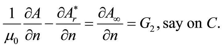(15)

These conditions, together with the vanishing condition at infinity of, are sufficient for the complete determination of the two harmonic functions A and.

The magnetic field components are expressed as

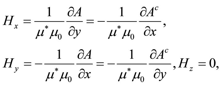(16)

where A^c denote the harmonic conjugate to A. It follows from (16) that the function plays the role of a scalar magnetic potential. Thus, one may invariably proceed with the problem formulation using either the magnetic scalar or the magnetic vector potential. We shall use the latter.

The solution of the electromagnetic problem thus reduces to the determination of two harmonic functions A, , subject to the boundary conditions (14) and (15).

2.1.2. Equations of Elasticity

1) Equations of equilibrium.

In the absence of body forces of non-electromagnetic origin, the equations of mechanical equilibrium in the plane read

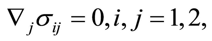(17)

where are the components of the “total” stress tensor and denotes covariant differentiation. It is worth noting here that the total stress tensor is sometimes decomposed into two parts: mechanical and electromagnetic [10], in which case the boundary conditions may take different forms.

It is well-known that Equation (17) is satisfied if the only identically non-vanishing stress components, and are defined through the stress function U by the relations

(18)

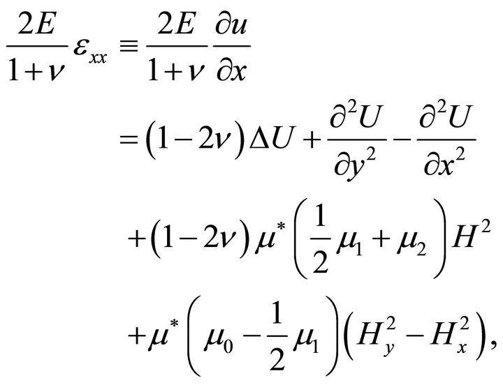
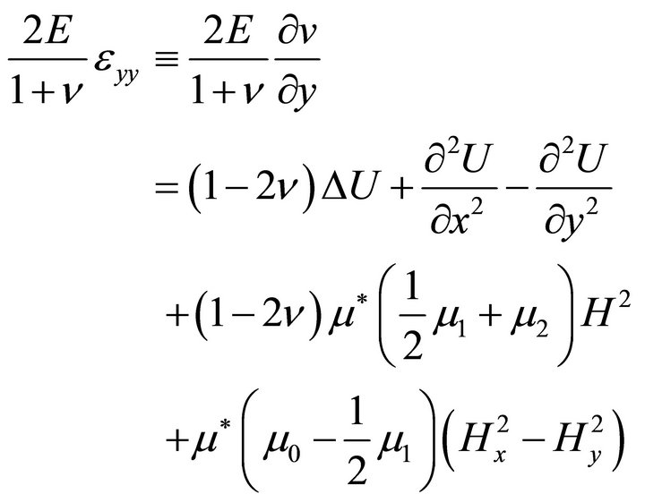
2) The constitutive relations.

The generalized Hooke’s law may be derived consistently for an appropriate form of the free energy of the medium, using the general principles of Continuum Mechanics. It reads [8, see also 9 for the electric analogue]

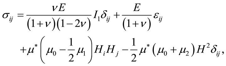(19)

where 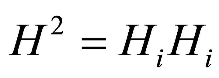is the squared magnitude of the magnetic field. In components, Equation (19) gives

(20a)

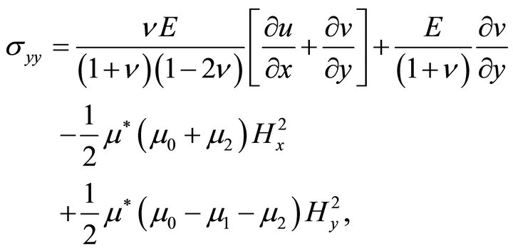(20b)

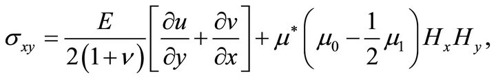(20c)

where are Young’s modulus and Poisson’s ratio respectively for the considered elastic medium.

3) The kinematical relations.

These are the relations between the strain tensor components and the displacement vector components.

(21a)

or, in Cartesian components

(21b)

where and stand for and respectively.

4) The compatibility condition.

The condition of solvability of Equation (21b) for and for given R.H.S. is

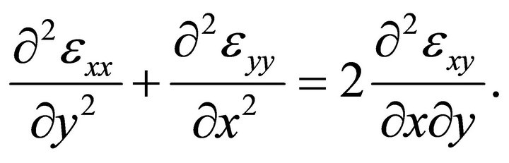(22)

These equations are complemented with the proper boundary conditions, to be discussed in detail in subsequent sections.

Equation for the stress function

An equation for the stress function may be obtained from the general field equations written in covariant form [11]. For the present purposes, however, we prefer to derive this equation for the special, two-dimensional problem under consideration. Solving (20) for the strain components and using (18), one obtains

(23a)

(23b)

and

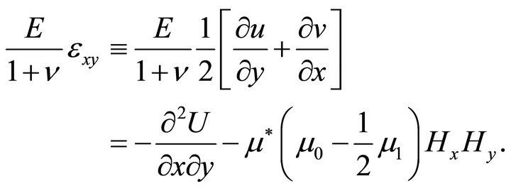(23c)

Substituting from (23) into (22) and performing some transformations using the equations of Magnetostatics and (3), one finally arrives at the following inhomogeneous biharmonic equation for the stress function:

(24)

The solution of (24) is sought in the form

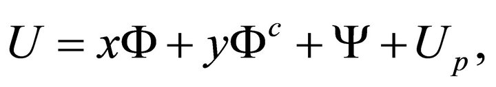(25)

where and are harmonic functions belonging to the class of functions, denotes the closure of D and superscript “c” denotes the harmonic conjugate. Function is any particular solution of the equation

(26)

and may be expressed in the form of Newton’s potential after the function on the R.H.S. has been determined.

It follows from (25) that

(27)

Using Equations (25) and (27), Equations (23a,b) may be cast in the form

(28a)

and

(28b)

where

(29a)

and

(29b)

Function is defined up to an additive arbitrary constant, which may be determined by fixing the value of the function at an arbitrarily chosen point of.

Introducing two new functions

(30a)

and

(30b)

it can be easily verified using the equations of Magnetostatics that

(31a)

and

(31b)

Equations (31), imply the existence of two singlevalued functions and in D such that

(32a)

and

(32b)

with these notations, equations (28a,b) take the form

(33a)

and

(33b)

It is to be noted that the addition of a constant to the function amounts to adding linear terms in y to and linear terms in x to, which do not alter (33a,b).

A representation for the mechanical displacement vector components

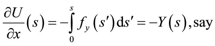
Differentiating (33a) w.r.t. y and integrating the resulting equation w.r.t. x after using (31a) and (32a), one gets

(34a)

where is an arbitrary function of y.

A similar procedure with (33b), using (31b) and (32b), yields

(34b)

where is an arbitrary function of x.

Substituting from (34a,b) into (23c), we find that this equation is identically satisfied if and only if

from which it follows that both functions are constants and therefore may be eliminated since their contribution represents a rigid body displacement. A similar argument holds for any constant added to the expression for. For the following procedure, it will be assumed that each one of these two functions has been completely determined by assigning to it a given value at some arbitrarily chosen point in.

From (33a) and (34a) once, then from (33b) and (34b), by line integrations along any path inside the region D joining an arbitrary chosen fixed point (which may be arbitrarily chosen in) to a general field point M, one obtains

(35a)

and

(35b)

where

(35c)

and

(35d)

the integration constants being absorbed into functions and which are yet to be determined.

The mechanical displacement components u and v given by expressions (35a,b) are single-valued functions in D, since the line integrals in (35c,d) are path independent due to relations (32a,b).

3. Boundary Integral Representation of the Solution

The problem now reduces to the determination of seven harmonic functions: and (although the conjugate function does not appear in the expressions given above for the stress and displacement functions, it will be required for the subsequent analysis within the proposed boundary integral method).

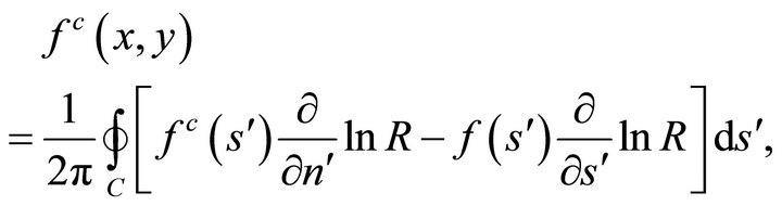
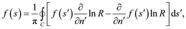
We use the well-known integral representation of a harmonic function f at a general field point inside the region D in terms of the boundary values of the function and its harmonic conjugate (after integrating by parts and rearranging) as

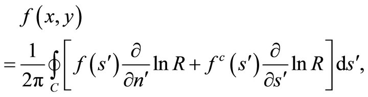(36a)

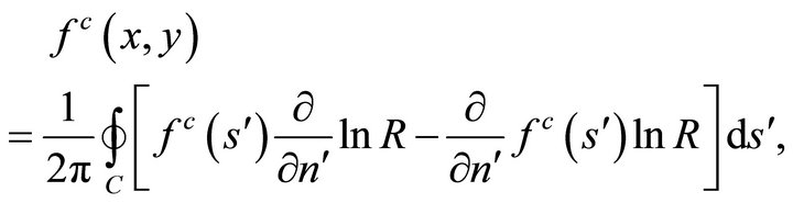
or, in the equivalent form

(36b)

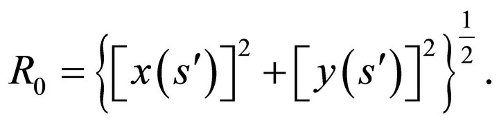
where is the distance between the field point in and the current integration point on.

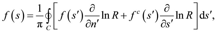
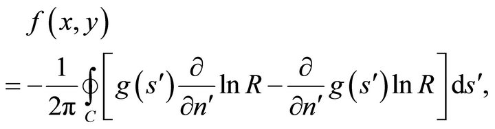
The harmonic conjugate of (36b) is

(36c)

where

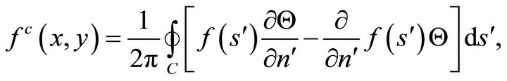
The representation of the conjugate function is given by

(37a)

or, in the equivalent form

(37b)

when point tends to a boundary point, relations (36a) and (36b) are respectively replaced by

(38a)

and

(38b)

If a function is defined in the outer region, is harmonic in this region and vanishes at infinity at least as with, it can be shown that the integral representation (36b) is replaced by

(39a)

it being understood that the boundary values and

under the integral sign on the R.H.S. are calculated at a point with parameter on the outer side of.

When the point tends to a boundary point with parameter s, then (39a) is replaced by the integral relation

(39b)

3.1. Solution for the Magnetic Vector Potential

As noted above, each of the two functions and is defined up to an arbitrary constant, to be fixed by assigning a given value to the function at an arbitrarily chosen point in its domain of definition.

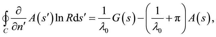
In order to obtain the boundary values of the two harmonic functions A and, write down equation (38b)

for and equation (39b) for then use the boundary conditions (14) and (15) to finally get the following integral equation for:

(40)

where

(41a)

and

(41b)

Equation (40) is the canonical form of the well-known linear Fredholm integral equation of the second kind for the determination of the boundary values of. Having solved this integral equation, the boundary values of may then be obtained from (25a). Also, using

(40) and its solution, Equation (38b) written for is reduced to the following Fredholm integral equation of the first kind for the normal derivative of this function:

(42)

the solution of which allows to determine on the boundary using the boundary condition (15). Thus, the boundary values of A and, as well as of their normal derivatives, may be determined.

Finally, Equations (36b) and (39a) yield the values of the magnetic vector potential everywhere in space, while Equation (36c) gives the harmonic conjugate in the body.

3.2. Solution for the Stress and Displacement Components

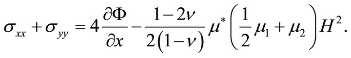
Having obtained the solution for the magnetic field everywhere in space and in the region D occupied by the material, we now turn to solve the mechanical problem for the stress and the displacement components in. The stresses are given through the stress function from relations (20a,b,c), and these may be rewritten using expression (25) in terms of the harmonic functions and the particular solution in the form

(43a)

(43b)

(43c)

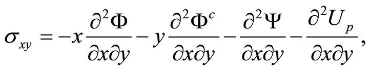
from which, using (21), one obtains

(44)

Thus, once the magnetic field has been uniquely determined, the derivative must be a uni-valued function.

The mechanical displacement components are given from relations (35a,b), which may rewritten using (25) in terms of the harmonic functions and as

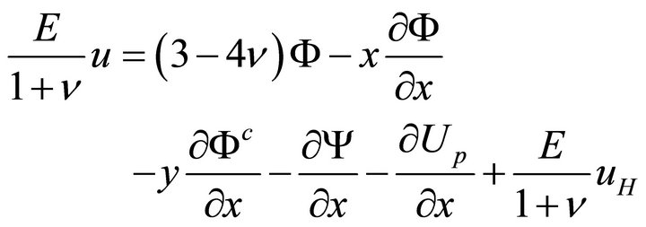(45a)

and

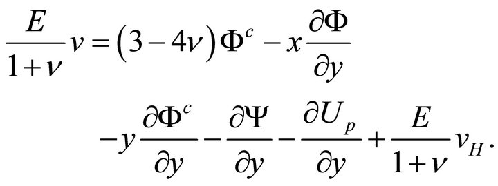(45b)

In view of the integral representations (37a,b) and expressions (43) and (45), it is sufficient for the solution of the mechanical problem to determine the boundary values of the harmonic functions and. This requires four independent relations in these unknowns, two of which are obtained from relation (38a) written for and and the remaining two from the boundary conditions. As a matter of fact, other conditions will still be required to eliminate the possible rigid body motion. Following [5], we formulate the conditions for the two following fundamental problems: The first fundamental problem, where the stresses are specified on the boundary, and the second fundamental problem, where the displacements are specified on the boundary.

4. Conditions for the Uniqueness of the Solution

4.1. Conditions for Eliminating the Rigid Body Translation

Following [5],

(46a)

and

(46b)

In terms of the boundary values of the unknown harmonic functions, condition (46) becomes

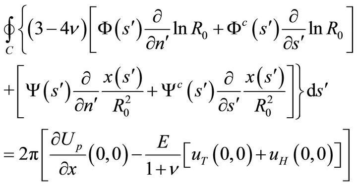(47a)

and

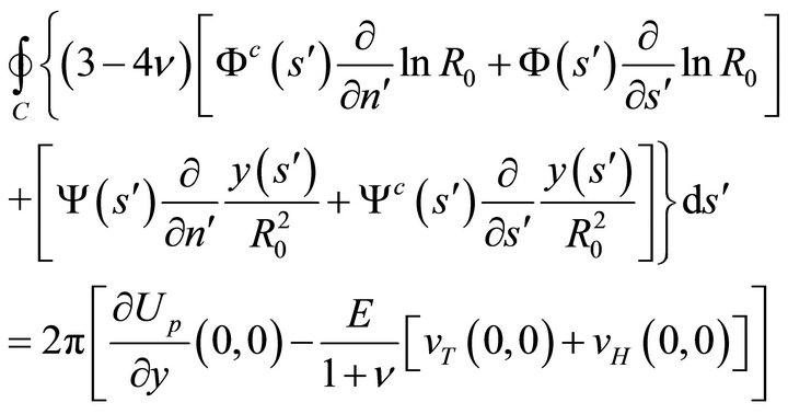(47b)

where

4.2. Conditions for Eliminating the Rigid Body Rotation

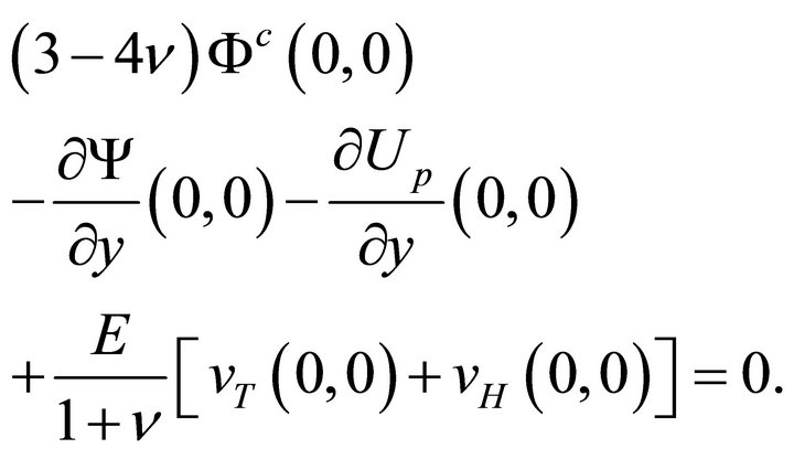
This condition, like the first two, is applied only for the first fundamental problem. We shall require that

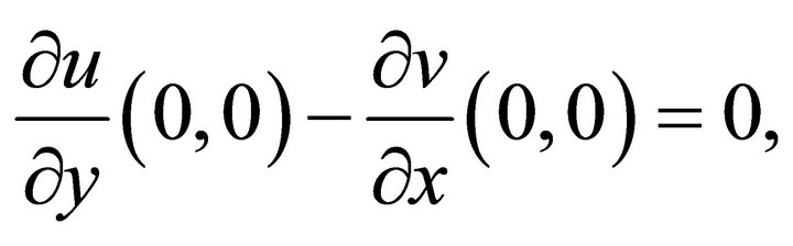
or, using (45),

(48)

which may be written in terms of the boundary values of the unknown harmonic functions as

(49)

4.3. Additional Simplifying Conditions

We shall require the following supplementary conditions to be satisfied at the point of the boundary, in order to determine the totality of the arbitrary integration constants appearing throughout the solution process. These additional conditions have no physical implications on the solution of the problem. For details concerning these additional conditions, the reader is kindly referred to [3].

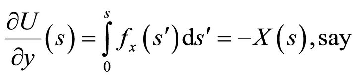
1) The vanishing of the function U and its first order partial derivatives at

(50a)

or, equivalently,

(50b)

which, in terms of the boundary values of the unknown harmonic functions, give

(51a)

(51b)

and

(51c)

2) The vanishing of the combination

(51d)

This last additional condition amounts to determining the value of at and is chosen for the uniformity of presentation as in [5].

Let us finally turn to the boundary conditions related to the equations of Elasticity. For this, we consider separately two fundamental boundary-value problems.

4.3.1. The First Fundamental Problem

In this problem, we are given the force distribution on the boundary C of the domain D. Let

denote the external force per unit length of the boundary. Then, at a general boundary point Q the stress vector is taken to satisfy the condition of continuity

or, in components

(52)

The force is divided into two parts:

(53)

where is the force of non electromagnetic origin and is the force due to the action of the magnetic field, per unit length of the boundary. The second force may be expressed in terms of the Maxwellian stress tensor as

(54)

with

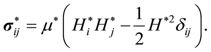(55)

Substituting for and in terms of the stress function and for and and taking conditions (51) into account, the last two relations yield

(56a)

and

(56b)

Using expressions (56), one may easily obtain the tangential and normal derivatives of the stress function at the boundary point.

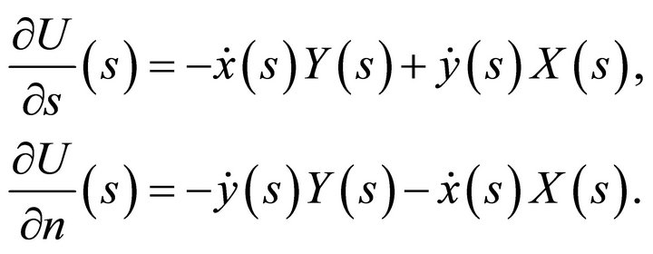(57)

or, in terms of the unknown harmonic functions

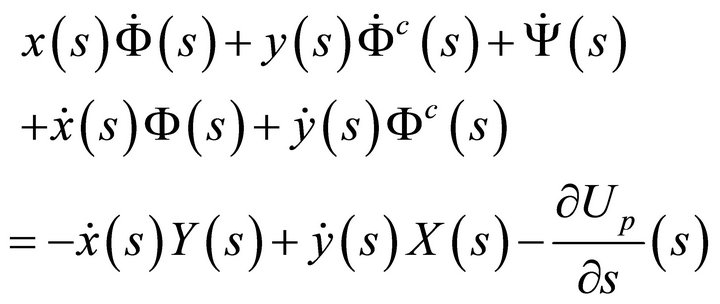(58a)

and

(58b)

Equations (58), together with relation (38) written for and:

(59a)

and

, (59b)

form a set of four integro-differential relations, the solution of which under the set of conditions (47), (48) and (51) provides the boundary values of the unknown harmonic functions and and their harmonic conjugates. The full determination of these functions inside the domain D (and hence of the biharmonic part of the stress function U) is then achieved by substitution into the Equation (37) written for and. The stress function U is finally obtained by adding up the particular integral.

4.3.2. The Second Fundamental Problem

In this problem, we are given the displacement vector on the boundary of the domain. Let this vector be denoted

Multiplying the restriction of expression (45a) to the boundary by and that of expression (45b) by and adding, one gets

(60a)

Similarly, if one multiplies the restriction of expression (45a) to the boundary by and that of expression (45b) by and subtracting, one obtains

(60b)

These last two relations may be conveniently rewritten as

(61a)

and

(61b)

where and are the tangential and normal components respectively, calculated at boundary points, of the vector, the Cartesian components of which are and given by equations (35c,d).

Equations (60a,b) (or (61a,b)), together with (59a,b) form the required set of simultaneous integro-differential equations for the determination of the boundary values of the unknown harmonic functions Φ and Ψ and their harmonic conjugates. The full solution of the problem proceeds as for the first fundamental problem.

4.4. Practical Use of the Method

In practice, if the form of the boundary is simple enough (e.g. the circle or the ellipse), one may attempt to find analytical forms for the solution as shown below in the application. However, for more complicated boundaries, one has to recur to numerical approaches. In this casethe differential and integral operators appearing in the equations are to be discretized as usual and the problem of determination of the boundary values of the unknown functions reduces to finding the solution of a linear system of algebraic equations. The full solution inside is then obtained by numerical integration of boundary integrals of the type (36) [cf. 6,7].

In a later stage, if it is required to determine boundary values of some unknown functions (for example, the boundary displacement for the first fundamental problem or the boundary stresses for the second fundamental problem), this may be achieved at once if the solution is obtained analytically as in the worked examples. Otherwise, if a numerical approach is adopted, the calculation may proceed by calculating the first and the second derivatives w.r.t. and of the required functions on the boundary in terms of derivatives taken along the boundary and then substituting these into the proper expressions (for example, expressions (43) for the stresses and (45) for the displacements).

5. The Circular Cylinder

As an illustration of the proposed scheme, we present here below the solution of a problem which can be handled analytically, namely the infinite, non-conducting, circular elastic cylinder placed in a transverse constant external magnetic field.

Let the normal cross-section of the cylinder be bounded by a circle of radius centered at the origin of coordinates, with parametric equations

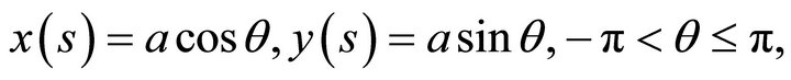
where is the polar angle in the associated polar system of coordinates.

Let a circular cylinder of a weak electric conducting, magnetizable material be placed in an external, transversal constant magnetic field, which we take along the -axis.

5.1. Solution for the Equations of Magnetostatics

The solution for the magnetic vector potential component is obtained following steps similar to those of the preceding section in the form:

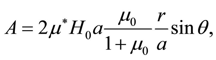(62a)

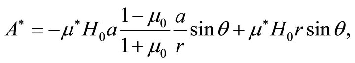(62b)

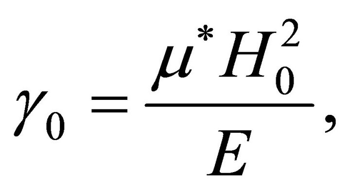
where is the intensity of the applied magnetic field.

The linear part in r in the expression for A^* is just the function in the general formulation of the problem.

Choosing to vanish at the origin, one gets

(62c)

The corresponding magnetic field components are

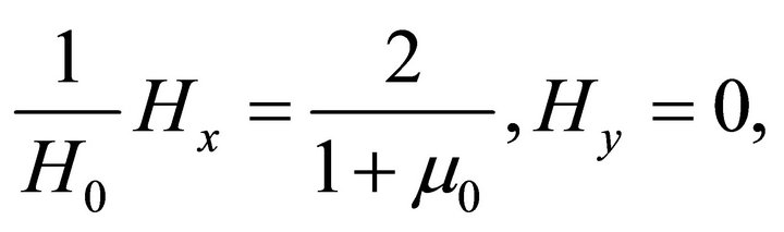(63a)

(63b)

or, related to the system of polar coordinates

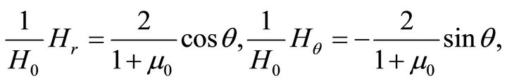(64a)

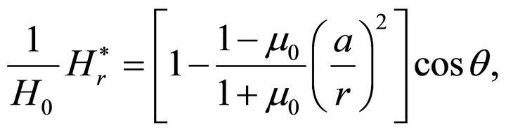(64b)

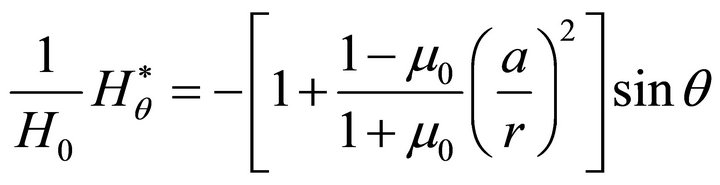(64c)

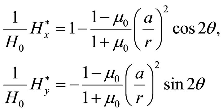
Also,

(65a)

(65b)

The boundary values of the magnetic field outside the body are used to calculate the Maxwellian stress tensor components for the formulation of the boundary conditions of elasticity. One obtains

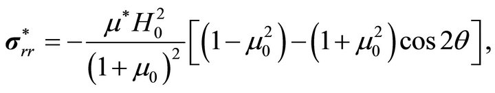(66a)

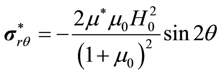. (66b)

5.2. The Elastic Solution

Turning now to the determination of the stresses and displacements, one has

where we have introduced the dimensionless parameter

from which one obtains

(67)

with

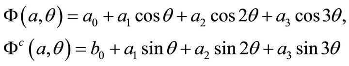
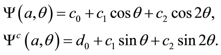
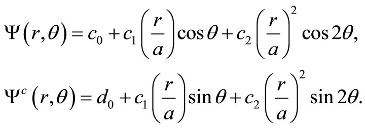
The restrictions of the functions and and of their harmonic conjugates to the boundary are expressed as general Fourier expansions in the polar angle of the system of polar coordinates. For the case under consideration:

and

Inside the body:

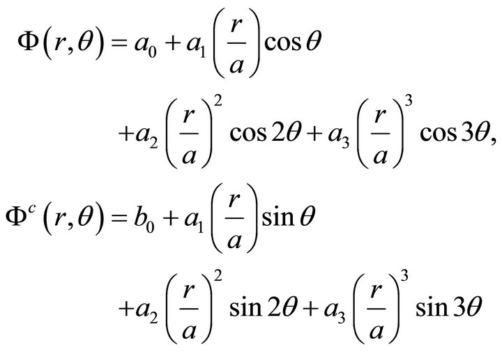
and

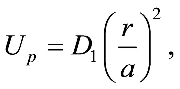
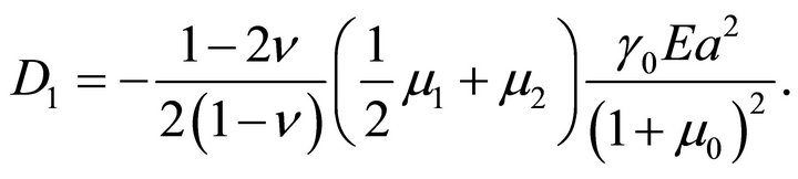
The stress function inside the domain is then

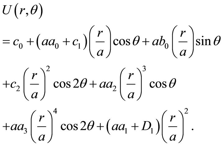(68)

The four simplifying conditions taken at the point yield

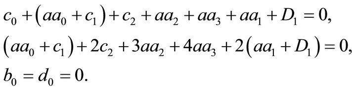
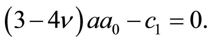
Of the two conditions expressing the suppression of the rigid body translation, one is identically satisfied, while the other gives

The suppression of the rigid body rotation is identically satisfied.

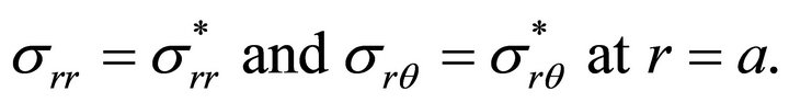
There remains now the boundary conditions to be satisfied, which may be simply written as the conditions of continuity of the two stress components and related to the system of polar coordinates:

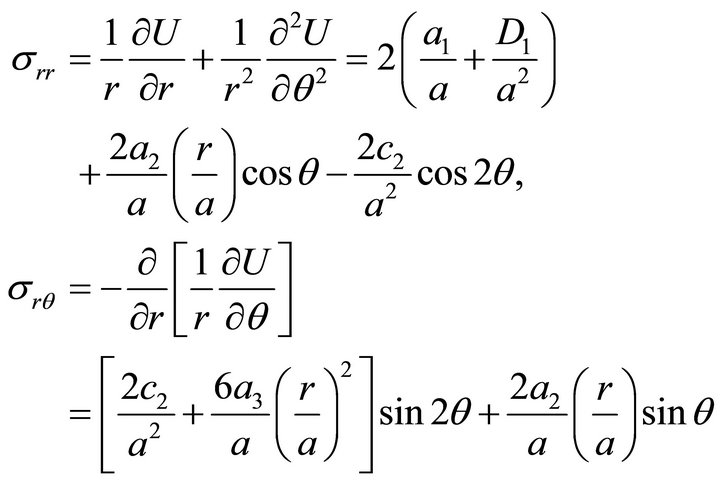
The stress components and may be calculated from in the polar system of coordinates as follows:

and

The first of the elastic boundary conditions then gives

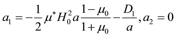
and

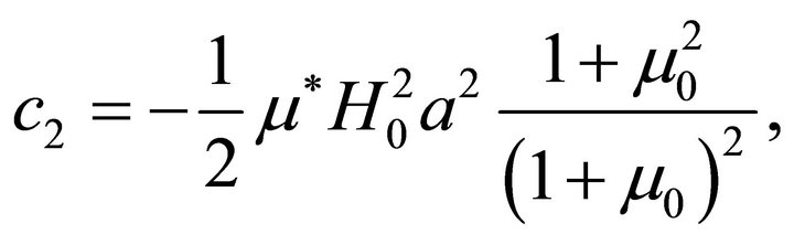
while the second one yields

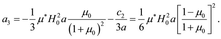
Finally,

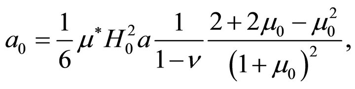
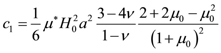
and

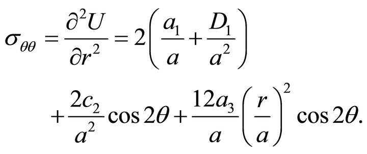
The stress components are

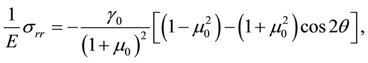(69a)

(69b)

and

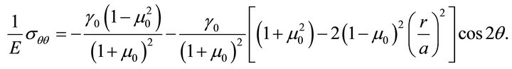(69c)

Finally, the mechanical displacement components are

(70a)

and

(70b)

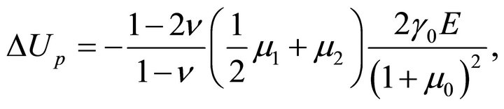
It is worth noting here that the material constants and appear only in the expression for the radial displacement. A measurement of this displacement at the surface of the cylinder provides the numerical value of the combination. The solution for the elliptical boundary could provide two different relations for the determination of both and.

6. Conclusion

The plane problem of linear, uncoupled Magnetoelasticity for the case of an external, transversal magnetic field in the absence of current has been tackled using a boundary integral formulation developed earlier by the authors and tested in the simpler cases of pure elasticity, uncoupled thermoelasticity and magneto-thermoelasticity in the presence of axial current. The presented theory and the application concerning the circular boundary clearly point out at the efficiency of the method in providing analytical solutions whenever this is possible.

REFERENCES

- M. S. Abou-Dina and A. A. Ashour, “A General Method for Evaluating the Current System and Its Magnetic Field of a Plane Current Sheet, Uniform Except for a Certain Area of Different Uniform Conductivity, with Results for a Square Area,” Il Nuovo Cimento C, Vol. 12, No. 5, 1989, pp. 523-539.
- M. S. Abou-Dina and M. A. Helal, “Reduction for the Nonlinear Problem of Fluid Waves to a System of Integro-Differential Equations with an Oceanographical Application,” Journal of Computational and Applied Mathematics, Vol. 95, No. 1-2, 1998, pp. 65-81. doi:10.1016/S0377-0427(98)00072-7
- M. S. Abou-Dina and A. F. Ghaleb, “On the Boundary Integral Formulation of the Plane Theory of Elasticity with Applications (Analytical Aspects),” Journal of Computational and Applied Mathematics, Vol. 106, No. 1, 1999, pp. 55-70.
- M. S. Abou-Dina and A. F. Ghaleb, “On the Boundary Integral Formulation of the Plane Theory of Thermoelasticity (Analytical Aspects),” Journal of Thermal Stresses, Vol. 25, No. 1, 2002, pp. 1-29. doi:10.1080/014957302753305844
- M. S. Abou-Dina and A. F. Ghaleb, “On the Boundary Integral Formulation of the Plane Theory of ThermoMagnetoelasticity,” International Journal of Applied Electromagnetics and Mechanics, 11, No. 3, 2000, pp. 185- 201.
- M. S. Abou-Dina and A. F. Ghaleb, “On the Boundary Integral Formulation of the Plane Problem of Elasticity with Applications (Computational Aspects),” Journal of Computational and Applied Mathematics, Vol. 159, No. 2, 2003, pp. 285-317.
- J. A. El-Seadawy, et al., “Implementation of a Boundary Integral Method for the Solution of a Plane Problem of Elasticity with Mixed Geometry of the Boundary,” Proceedings of the 7th International Conference on Theoretical and Applied Mechanics, Cairo, 11-12 March 2003.
- L. D. Landau, E. M. Lifshitz and L. P. Pitaevskii, “Electrodynamics of Continuous Media,” 2 Edition, Pergamon Press, Oxford, 1984.
- R. J. Knops, “Two-Dimensional Electrostriction,” The Quarterly Journal of Mechanics and Applied Mathematics, Vol. 16, No. 3, 1963, pp. 377-388.
- K. Yuan, “Magnetothermoelastic Stresses in an Infinitely Long Cylindrical Conductor Carrying a Uniformly Distributed Axial Current,” Journal of Applied Sciences Research, Vol. 26, No. 3-4, 1972, pp. 307-314.
- M. M. Ayad, et al., “Deformation of an Infinite Elliptic Cylindrical Conductor Carrying a Uniform Axial Current,” Mechanics of Materials, Vol. 17, 1994, pp. 351-361.