Engineering
Vol. 3 No. 3 (2011) , Article ID: 4148 , 4 pages DOI:10.4236/eng.2011.33031
Prediction of Shear Wave Velocity in Underground Layers Using SASW and Artificial Neural Networks
Faculty of Mining, Petroleum and Geophysical Engineering, Shahrood University of Technology, Shahrood, Iran
E-mail: andisheh@mine.tus.ac.ir
Received December 6, 2010; revised January 6, 2011; accepted February 9, 2011
Keywords: Shear Wave Velocity, SASW, DHT, Neural Networks, Geotechnical Investigations
ABSTRACT
This research aims at improving the methods of prediction of shear wave velocity in underground layers. We propose and showcase our methodology using a case study on the Mashhad plain in north eastern part of Iran. Geotechnical investigations had previously reported nine measurements of the SASW (Spectral Analysis of Surface Waves) method over this field and above wells which have DHT (Down Hole Test) result. Since SASW utilizes an analytical formula (which suffers from some simplicities and noise) for evaluating shear wave velocity, we use the results of SASW in a trained artificial neural network (ANN) to estimate the unknown nonlinear relationships between SASW results and those obtained by the method of DHT (treated here as real values). Our results show that an appropriately trained neural network can reliably predict the shear wave velocity between wells accurately.
1. Introduction
Shear wave velocity estimation is an important task due to its application in evaluating sub surface response to earthquakes, soil improvement, and the strength of the surface structures’ foundation. Two common methods for determining shear wave velocity profile in sub surface layers are Down Hole Test (DHT) and Cross Hole Test (CHT). As a weak point, in these methods we need to drill bore holes. Bore hole drilling is a destructive, expensive and time consuming task. Therefore a proper non-destructive alternative for these methods is needed. Spectral analysis of surface waves (SASW) method is a non destructive procedure which gives shear wave velocity using seismic surface waves [1].
Instead compressional body waves (P) and shear waves (S), there is the other wave which propagates on the surface of the medium. This wave called Rayleigh Wave. Its velocity is less than shear wave. This wave can be produced by hammer or weighted drop. In 1984 a non destructive method was developed which called Spectral Analysis of Surface Waves (SASW) [2].
The first step in SASW method is data acquisition. By vertical impact to the surface of the ground, Rayleigh waves will propagate. These waves have a special frequency range and are recorded by two geophones lied on the line through the surface. The distance between geophones should be increased symmetrically with respect to the mid point of the geophones. Then it is possible to obtain the dispersion curve (phase velocity as a function of propagated wave frequency) in the next step. Common array of source and geophones is shown in Figure 1.
The second step is data processing. In this step, the phase difference between two signals recorded with geophones (x(t) and y(t)) is obtained. This phase difference is a function of Rayleigh wave frequency which propagates the distance between two geophones. To calculate the phase difference, signals from time domain should transfer to the frequency domain using Discrete Fourier Transform. After that X(f) and Y(f) are obtained. Therefore Cross Power Spectrum Function (GYX) and the phase are calculated using Equations (1) and (2).
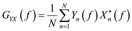 (1)
(1)
Here X*(f ) is a Complex Conjugate of X(f ).
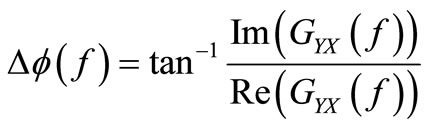 (2)
(2)
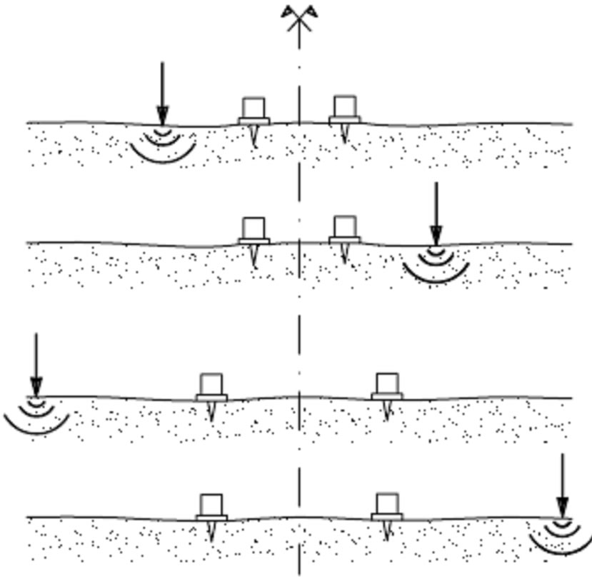
Figure 1. Array of source and geophones [3].
Calculated phase from Equation (2) is a phase difference between X(f ) and Y(f ).
Using Equation (3), we can calculate the dispersion curve.
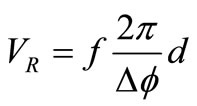 (3)
(3)
In step 3 we should determine shear wave velocity profile (VS versus depth). Considering that shear wave velocity is approximately equal to 1.1 VR, so VS can be obtained. Also the effective penetration depth of Rayleigh waves is equal to , so D (depth) can be obtained too [3].
2. Methodology
2.1. Seismic Data Acquisition
The proposed methodology is explained using a realistic example. Nine SASW measurements performed over the Mashhad Plain in north eastern part of Iran [4]. All of the measurements performed above bore holes which had DHT results. Figure 2 shows the geological map of the Mashhah Plain. In this figure, BH means bore hole and black dots illustrate the position of nine bore holes.
SASW measurements are VS (Shear Wave Velocity),  (Unwrap Phase Differences), f (Frequency), d (Distance between Geophones), and D (Depth of Evaluation). These parameters are reported for bore hole 19 (BH19) in Table 1.
In Table 1, values of the fifth column are shear wave velocities from DHT method, which are treated as the real values.
Figure 2. Geological map of the Mashhad Plain [5].
Table 1. Data obtained from SASW and DHT from depth 1.0353 m to 2.2726 m in BH19.
2.2. Problem Statement and Solution Strategy
As mentioned in Table 1, shear wave velocity values measured with both SASW and DHT methods for all 9 bore holes. Figure 3 illustrates the comparison of these values for various depths in each bore hole. If we assume the values of shear wave velocity from DHT method as the real values, it will obvious that SASW have a relatively good estimation when the prediction depth is shallow. By increasing in depth values, the accuracy of SASW estimations will fall in doubt. These differences in shear wave velocity estimation can be because of the existence of noise and unknown non linear relationships between SASW results and real values of shear wave velocity. Recognizing the computational power of artificial neural networks in rule generation and function approximation and their robustness particularly in the area of data classification, we embarked on development and training of a back-propagating artificial neural network (BP) for the purpose of classification of shear wave velocity considered in this study.
2.3. Back-Propagating Artificial Neural Networks (BANN)
Artificial neural networks (ANNs) are computational models based on human’s understanding of cortical structure of the brain and cognition. Algorithmically, ANNs are parallel adaptive systems and therefore require training. Back-propagation is a powerful method of supervised learning that is developed after the seminal work by Paul Werbos and David E. Rumelhart in seventies and eighties [6]. Details of various methods of ANN design and training are beyond the scope of this paper and are explained elsewhere (see [7] and [8] for example); nevertheless a brief description of the terminology is provided here.
The structure of a neural network, in general, consists of an interconnected group of artificial neurons (simple processors that are connected to many other neurons). These processing units receive the information, apply some simple processing on them and pass them to other neurons. The flow of information creates a computational

Figure 3. Small circle symbols illustrate the real values of shear wave velocity for each bore hole from DHT method while the triangles are the shear wave velocity values obtained from the SASW method.
model for information processing. Each neuron is assigned a weight that is changed adaptively to improve the performance of the network based on pairs of external and internal signals (training information, input-output mapping). Practically, neural networks may be used in nonlinear statistical data modeling, system identification, extraction of complex relationships between inputs and outputs of a system, and for pattern recognition.
The structure of a simple neural network is shown in Figure 4.
In addition to weight, each node (neuron) in the network is equipped with an activation function (or transfer function) that is part of the information processing unit of the neuron. The flow of information could be imagined from left to right, such that each neuron performs
Figure 4. A simple neural network consisting of input, hidden, and output layers (with 3, 4, and 2 nodes, respectively) [9].
the processing on the data in parallel with other neurons in the layer. The response of the network is compared at the terminating layer with a set of desired outputs and the weights of the neurons are thusly corrected following a training algorithm to minimize the output error. Issues with regards to the number of nodes per layer, number of layers, and the type of activation function that could be used are dealt with in the design of the architecture of the network. This is explained later on in this paper.
There are numerous methods of training of a neural network. Categorically these methods are grouped into three main classes: supervised learning, unsupervised learning, and reinforcement learning. In a supervised learning scheme, the network is provided with a set of examples in the input-output space:  and the goal of the training process is to find function f in a set of valid functions that could match the input/output pairs reliably. By doing so, the network becomes capable of making inferences in mapping that is implied by the training data. This procedure involves minimizing a cost function. The cost function is often defined as the mismatch between the network’s mapping and the actual data.
A commonly used cost function is the mean-squared error between the average of network’s output, f(x), and the target value y over all example pairs presented to the network. Minimizing this cost function in a gradient descent algorithm for a class of neural networks called Multi-Layer Perceptrons constitutes the basis of backpropagation algorithm [6].
In this study, we successfully developed and implemented a network with two hidden layers of 5 and 7 nodes respectively.
3. Results and Discussion
The minimum dataset is 142 data points for BH17 and maximum dataset is 269 data points for BH9. Table 2
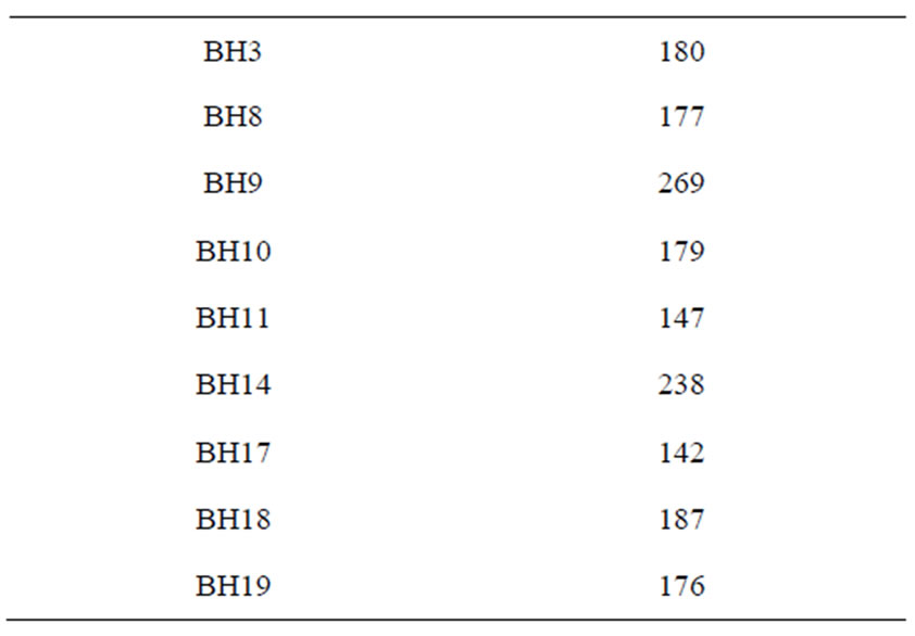
Table 2. Values of data points for each bore hole.
shows the values of data points for each bore hole.
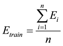
For each bore hole, we used it’s dataset to train and test the neural network. 70% of the total data points were selected randomly for the network training and the remaining 30% of the data was used for testing the network. Each data point is a vector of four input values, namely, d, f,  , and D as described earlier. The desired network output is real shear wave velocity value obtained from the DHT method (shown by small circles in Figure 3). The input layer of the network receives input data at four nodes and the network generates an output at the final layer. We used the Levenberg Marquardt (LM) algorithm for training method because it generally results in faster and more reliable convergence for our application. Average error values of 50 iterations for training and testing of the network for each bore hole data points are presented in Table 3. In Table 3, Etrain is the absolute error after network convergence, Etest is the error obtained from testing the network, RMStrain is the root-mean-square of the training error, and RMStest is the root-mean-square of error during testing of the network. Results shown in Table 3 appear to be very reasonable for practical applications.
The absolute training error Etrain is calculated in the following manner:
 (4)
(4)
and
 (5)
(5)
In Equation (4), r is the real shear wave velocity value, p is the predicted shear wave velocity value from the network, and n is the number of training data. Etest is as
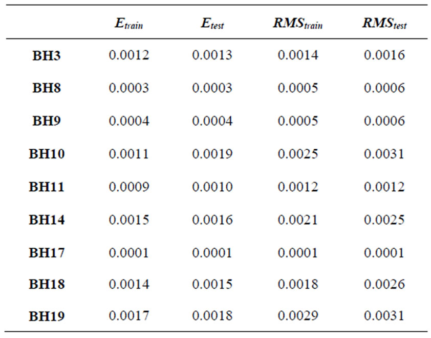
Table 3. Average error values for the training and testing the network in each bore hole.
the same as Etrain but is calculated from the test data. RMStrain is the mean square error of the training data and is obtained from Equation (6):
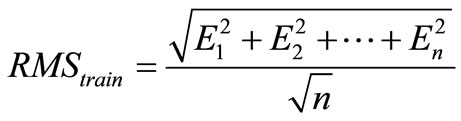 (6)
(6)
RMStest is calculated as RMStrain but for the test data.
From Table 3, the average RMS of the error for train and test results in each bore hole is near zero. The reduction in the network error will increase the reliability of network’s predictions. Other training algorithms such as Scaled Conjugate Gradient, One-Step Secant, and Fletcher-Powell Conjugate Gradient were also used but were discarded due to higher tolerance for the test errors and lower reliability in our application [4,6]. With a network of only one hidden layer, overtraining was often observed. Overtraining happens when the network is highly trained but its predictions appear erroneous for the test data. This can be the consequence of the complexity of problem investigated here and modeled in our neural network.
The results of the training for BH8 are presented in Figure 5.
In Figure 5, R is the correlation coefficient between the real and the predicted shear wave velocity values; A being the predicated and T being the real value. The correlation coefficient is 1.0, implying a very good network performance.
We used the abovementioned neural network for the task of classifying the test data. The results are shown in Figure 6.
During testing, a correlation coefficient of 1.0 was generally obtained (as exhibited in Figure 6). This shows that the shear wave velocity values in the test data were practically well-correlated with the network predictions. The problem with SASW method was its poor performance in estimating shear wave velocities in Mashhad Plain, therefore it deemed appropriate to be exceedingly meticulous with reliability of the computational tool that was developed as a part of this study to perform the task of classification. This is evident in Figure 7 with the superior performance of the trained network in BH8 (as opposed to the data Figure 3) remarkably demonstrated.
The real values of shear wave velocity, shown by small circles in Figure 7 could not be easily predicted by the SASW method but the back-propagating neural network, shown in Figure 7 by inverted triangles, quite consistently detected all shear wave velocities precisely.
The train and test results for other bore holes have been illustrated in Figures 8 and 9, respectively. From these figures it is obvious that the network has a very good performance in predicting shear wave velocities in another bore holes.
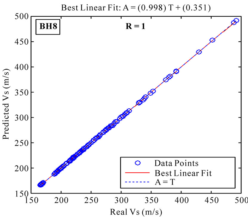
Figure 5. Correlation coefficient for train data in BH8.
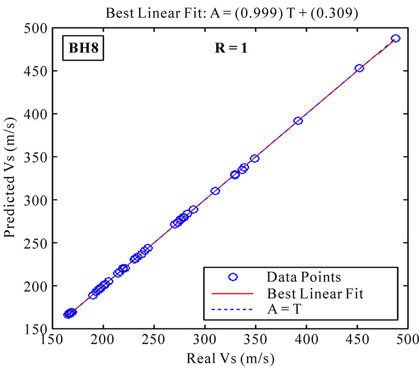
Figure 6. Correlation coefficient for the test data in BH8.
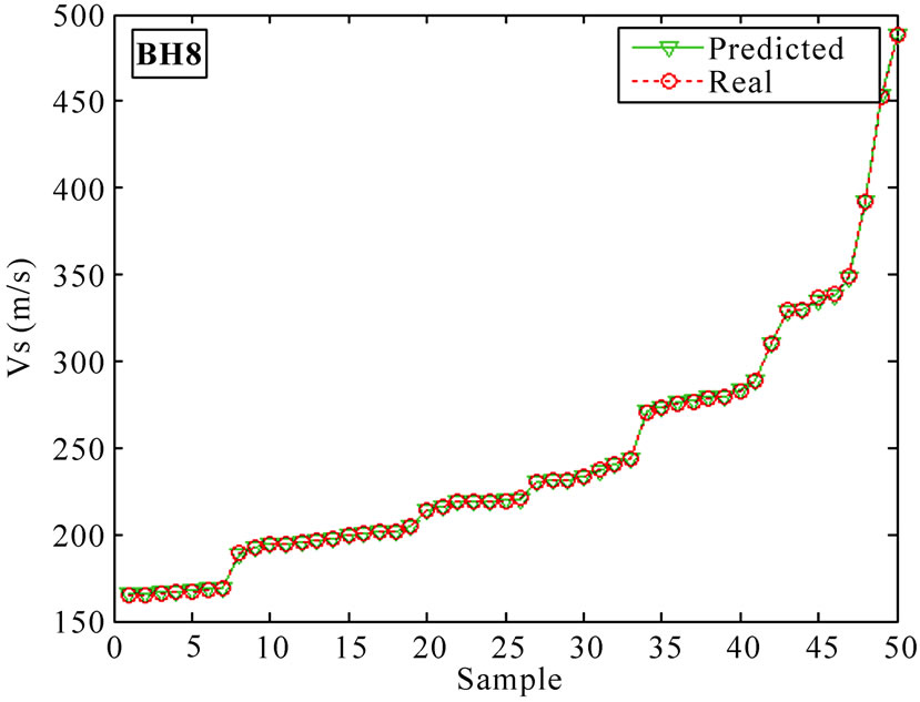
Figure 7. Predicted results for the test data in BH8.
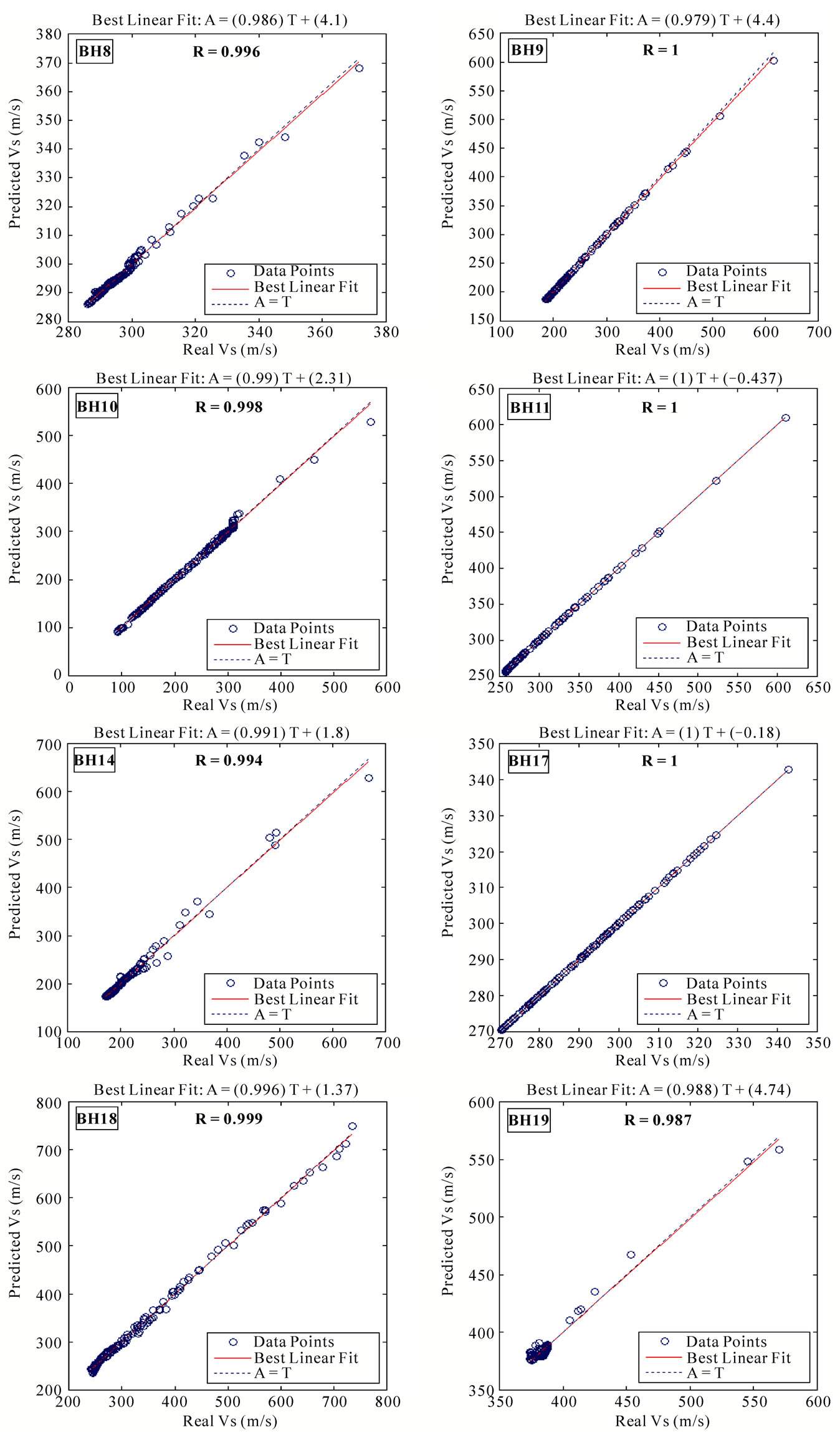
Figure 8. Train results for the other 8 bore holes.
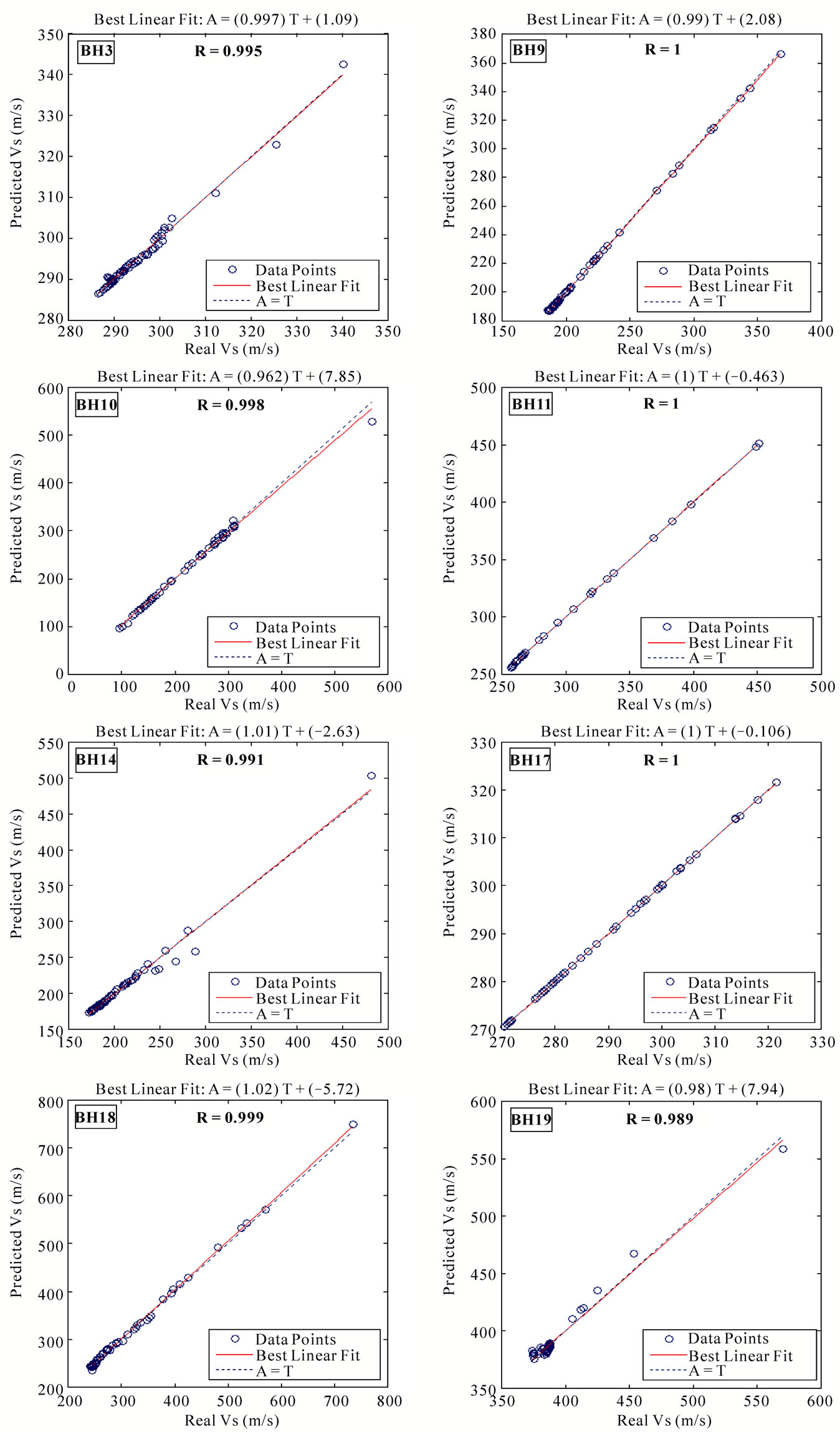
Figure 9. Test results for the other 8 bore holes.
4. Application of the Proposed Methodology to a Case Which Has Not Contributed in Training Procedure
Drilling holes is an expensive and time consuming task, so it is impossible to drill as many as holes that we need to obtain the detailed profile of shear wave velocity. Also in urban regions drilling is usually limited, therefore performing DHT method and getting real values of shear wave velocity for every desired point is not possible. Since in geostatistics it is possible to estimate an unknown point having its surrounding known points with the respect to their range of influence and their weights, it inspired us to estimate the shear wave velocities in a hole which has not contributed in the training procedure. Generalized Regression Neural Networks (GRNNs) are capable to do this. In these networks, each known point has its individual weight according to the assumed range of influence. Details of these networks are explained elsewhere (see [7] for example).
We selected five bore holes which were BH8, BH9, BH10, BH11, and BH14 respectively. According to Figure 2, BH9 is in the middle of the other four bore holes, so we considered it as the unknown hole. The network’s range of influence was 0.2 and the input data were the same as the back propagating neural network used for individual holes previously. We trained the network using the data of bore holes 8, 10, 11, and 14 and tested the trained network for bore hole 9. Figure 10 shows the shear wave velocity values from the SASW, DHT and those obtained from GRNN for the BH9.
In Figure 10, the trained neural network predicts lower shear wave velocity values (which SASW predicts them 100 m/s) perfectly. Interestingly in the middle part of this figure that SASW results are scatter, the GRNN can predict the values of shear wave velocity precisely. For higher depths the neural network predicts the lower values for shear wave velocities; but its estimation is still very better than SASW. We attribute this to the depth of investigation which impacts the seismic wave and reduces the ratio of signal to noise (S/N). Figure 10 illustrates that using SASW and GRNNs can predict the real values of shear wave velocity in the places in which it is impossible to drill holes.
5. Concluding Remarks
Measurement noise and nonlinear relationship between wave parameters and shear wave velocity quantities exert difficulties in performing seismic wave interpretation reliably. The SASW method, as a seismic-based nondestructive method, has been in use for some time and is susceptible to problems of predicting the shear wave velocities in underground layers. Consequently, other viable methods of prediction, such as the one proposed in this paper, may be deemed necessary in realistic cases. We successfully implemented and tested an artificially intelligent computational agent to consider the unknown nonlinear relationships between system variables in our prediction problem (foreseeing the shear wave velocities in underground layers). Our approach uses unwrap phase differences, frequency, distance between geophones, and depth of evaluation as input system variables. The network seeks the relationship between these input variables adaptively and strives to a desirable output which is, in our case, the real shear wave velocity values obtained
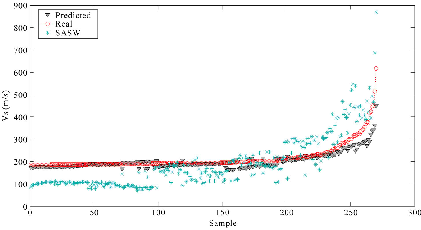
Figure 10. The shear wave velocity values from the SASW, DHT and those obtained from GRNN for the BH9.
from the down hole test method (DHT).
We considered two kinds of neural networks in our methodology. Back propagating artificial neural network used to predict the shear wave velocity values for each hole individually. The network could train itself very well with practically complete correlation between real shear wave velocity values and the predicted ones (correlation coefficient R of one). The network also exhibited a superior capability in estimating the unknown zones.
Applying the generalized regression neural network to predict the shear wave velocity values in a hole which had not contributed in the training procedure indicated that the network could perfectly predict the shear wave velocity values of lower and medium depths. Increasing the depth values, the network precision had a few decrease, but still it could give a very better results than SASW. We speculate the impact of decreasing in signal to noise ratio (S/N) as possible reason for this peculiarity.
Finally we could illustrate that it is possible to predict the values of shear wave velocity in places where it is impossible to drill holes. This can be achieved by drilling few wells in surrounding parts of the region, determining the real values of shear wave velocity (using DHT method), training a proper network (using SASW and DHT results), and applying the trained network in all over the region.
6. Acknowledgements
Authors would like to express their appreciation and gratitude to Dr. Hafezi Moghadas, for his help obtaining data. SASW and DHT data of the Mashhad Plain, used in this study were provided courtesy of Sahrakav Co.
7. REFERENCES
- V. Cuellar, “Geotechnical Application of the Spectral Analysis of Surface Wave,” Engineering Geology Special Publications, Geological Society, London, Vol. 12, 1997, pp. 53-62.
- A. M. Kaynia, “Spectral Analysis of Surface Wave (SASW),” Sort Course presented at the 3rd International Conference on Seismology and Earthquake Engineering, Tehran, 17-19 May 1999.
- S. Foti, “Multistation Methods for Geotechnical Characterization using Surface Waves,” Ph.D. Dissertation, Poletechnic di Torino, Torino, 2000.
- H. Shahsavani, “Application of SASW Method in Mashhad Plain,” M.Sc. Thesis, Shahrood University of Technology, Shahrood, 2007.
- N. H. Moghadas and A. Azadi, “Geoseismic Report of Mashhad Plain Microtremor Investigations,” Kavoshgaran Co., Tehran, 2006.
- H. Demuth and M. Beale, “Neural Network Toolbox for Use with MATLAB,” Version 3.0, 2002, pp. 1-742.
- M. T. Hagan, H. B. Demuth and M. Beale, “Neural Network Design,” PWS Publishing Company, Boston, 1996.
- J. C. Principe, N. R. Euliano and W. C. Lefebvre, “Neural and Adaptive Systems: Fundamentals through Simulations,” John Whily & Sons, New York, 1999, pp. 1-656.
- A. Alimoradi, A. Moradzadeh, R. Naderi, M. Z. Salehi and A. Etemadi, “Prediction of Geological Hazardous Zones in front of a Tunnel Face using TSP-203 and Artificial Neural Networks,” Tunnelling and Underground Space Technology, Vol. 23, No. 6, 2008, pp. 711-717. doi:10.1016/j.tust.2008.01.001