Engineering
Vol. 3 No. 4 (2011) , Article ID: 4598 , 4 pages DOI:10.4236/eng.2011.34043
Investigations on Non-Condensation Gas of a Heat Pipe
Department of Marine Engineering, National Taiwan Ocean University, Keelung, Taiwan, China
E-mail: jcwang@mail.ntou.edu.tw
Received October 29, 2010; revised December 8, 2010; accepted December 10, 2010
Keywords: Non-Condensation Gas, Heat Pipe, Maximum Heat Capacity
ABSTRACT
This paper utilizes numerical analysis method to determine the influence of non-condensation gas on the thermal performance of a heat pipe. The temperature difference between the evaporation and condensation sections of a single heat pipe and maximum heat capacity are the index of the thermal performance of a heat pipe for a thermal module manufacturer. The thermal performance of a heat pipe with lower temperature difference between the evaporation and condensation sections is better than that of higher temperature difference at the same input power. The results show that the maximum heat capacity reaches the highest point, as the amount of the non-condensation gas of a heat pipe is the lowest value and the temperature difference between evaporation and condensation sections is the smallest one. The temperature difference is under 1˚C while the percentage of the non-condensation gas is under 8 × 10⁻⁵%, and the heat pipe has the maximum heat capacity.
1. Introduction
The Thermal Management Control (TMC) is an important issue for the development and research of electronic device cooling technologies in the thermal module industry. A traditional cooler is fallible for a high power density heat source unless a two-phase heat transfer device, such as a heat pipe, is used. In 1963, Grover pointed out that a vacuum container generated lower amounts of oxygen if a copper pipe has the capillarity wick inside and fills the amount of pure water to treat as the working fluid [1]. After being heated, water in the hot end of the heat pipe evaporates as vapor that flows toward to the cooling end. The vapor dissipates heat from the heat source to the external environment and then condenses as liquid. The water reflows back to the hot end again because of the capillary force of the wick structure, so it completes the circulation of the heat exchange. Due to the circulation, the heat pipe may appear to decrease the temperature of the heat source under a minimal temperature difference, transfer the massive heat, and thereby make application in the industry of an electronic thermal module.
Due to the features of the heat pipe with high thermal conductivity and gravity, the thermal resistance is very low at appromaxiately 10−1 ˚C/W-10−3 ˚C/W [2-4]. Antigravity is another characteristic of a heat pipe, resulting from the capillary force of the wick structure; the optimum design of which can be obtained by using a nonlinear programming approach [5,6]. In 1987, Peterson et al. utilized the Maxwell and the Dul’nev method for the explanation of effective thermal conductivity functions of sintered powder thermal conductivity and the working fluid of thermal conductivity and porosity [7]. In 1995, Mohamed et al. [8] leaned the heat pipe, filled with water and composed of copper, to investigate its transition response. According to the different condensation rates and the heat source power input, the author directly gauged the axial temperature distributions of the integral heat pipe. The experiment demonstrated that the azimuth is insignificant to the time-constant influence. Each heat pipe’s heat capacity of the test facility which corresponds to the time-constant is different. A heat sink with embedded heat pipe has adequate thermal performance and low manufacturing cost implications in servers, PCs and notebooks [9,10]. The embedded heat pipes result in high effective thermal conductivity [11]. Gernert et al. used a heat sink with embedded heat pipes composed of a 25.4 mm diameter heat pipe and an aluminum heat sink [12]. When the maximum heat flux was 285 W/cm2, the minimum total thermal resistance value was 0.225 ˚C /W. Wang used an aluminum heat sink with embedded duo and quad heat pipes of 6 mm in diameter each [13]. The author carried 36% and 48% of the total dissipated heat away from the CPU while the total thermal resistance was under 0.24 ˚C/W. And Wang [14] also described the design, modeling, and test of a heat sink with embedded L-shaped heat pipes and plate fins including a windowsbased computer program using an iterative superposition method to predict the thermal performance. It is augmented with measured values for the heat pipe thermal resistance, which was within 5% of the measured value. The result of this work is a useful thermal management device along with a validated computer aided tool to facilitate rapid design. Therefore, the thermal performance of a heat pipe must be considered by its influence factor on the experiment, modifying its experimental parameters again in order to obtain the optimal performance of the heat pipe.
The first research using a set of the heat pipe with the experimental test was done by employing a subset which is compared with the numerical results and causes of the deviation between the numerical solution and the experimental data within an acceptable range [15]. According to the parameters of the simulation analysis as the input condition, the study considers other experimental results to confirm the accuracy of the simulated results. Final steps include revising the influence factor parameter, repeating the numerical analysis comparison, and finding the optimal parameter of the heat pipe. In this paper, applying the procedure of CFD simulation analysis to the thermal performance of the heat pipe can be adopted as a design method to investigate the different types of heat pipe and the optimum thermal performance of the thermal module.
2. Content
2.1. Heat Pipe
2.1.1. Principle
The heat pipe may mainly be differentiated for the evaporation section, the adiabatic section, and the condensation section and be regarded as the passive component of a self-sufficient vacuum closed system. The system which includes the capillarity structure and the filling of working fluid usually needs to soak through the entire capillarity structure. The fundamental construction of the traditional heat pipe is shown in Figure 1. When the heat pipe works, the evaporation section of the heat absorption occurs in the capillarity structure. The working fluid gasifies as the vapor. The high temperature and pressure vapor is produced at the condensation section after the adiabatic section. The vapor releases heat and then condenses as the liquid. The working fluid in the condensation section is brought back to the evaporation section because of the capillary force in the capillarity structure.
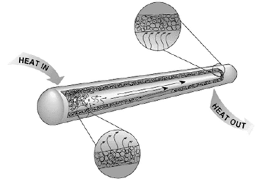
Figure 1. The basic structure of convectional heat pipe [2].
The capillary force has a relation with the capillarity structure, the viscosity, the surface tension, and the wetting ability. However, the capillary force and the high vapor pressure are the main driving force to make the circulation in the heat pipe. The working fluid in the heat pipe exists in the two-phase model of the vapor and liquid. The interface of the vapor and liquid’s coexistence is regarded as the saturated state. It is usually assumed that the temperatures of the vapor and liquid are equal.
2.1.2. Feature
The heat pipe uses the working fluid with much latent heat and transfers the massive heat from the heat source under minimum temperature difference. Because the heat pipe has certain characteristics, it has more potential than the heat conduction device of a single-solid-phase. Firstly, due to the latent heat of the working fluid, it has a higher heat capacity and uniform temperature inside. Secondly, the evaporation section and the condensation section belong to the independent individual component. Thirdly, the thermal response time of the two-phase-flow current system is faster than the heat transfer of the solid. Fourthly, it does not have any moving components, so it is a quiet, reliable and long-lasting operating device. Finally, it has characteristics of smaller volume, lighter weight, and higher usability.
2.1.3. Operating Limits
Although the heat pipe has good thermal performance for lowering the temperature of the heat source, its operating limitation is the key design issue called the critical heat flux or the greatest heat capacity quantity. Generally speaking, we should use the heat pipe under this limit of the heat capacity curve. There are four operating limits which are described as following.
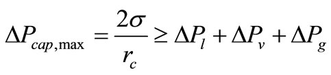
Firstly, the capillary limit, which is also called the water power limit, is used in the heat pipe of the low temperature operation. Specific wick structure which provides for working fluid in circulation is limiting. It can provide the greatest capillary pressure which is defined as
 (1)
(1)
where  is the maximum capillary pumping pressure,
  is surface tension (N/m),
  is effective capillary radius (m),
  is the pressure drop of liquid flow (Pa),
  is the pressure drop of vapor flow (Pa), and
  is the pressure drop due to gravity (Pa).
Secondly, the sonic limit is that the speed of the vapor flow increases when the heat source quantity of heat becomes larger. At the same time, the flow achieves the maximum steam speed at the interface of the evaporation and adiabatic sections. This phenomenon is similar to the flux of the constant mass flow rate at conditions of shrinking and expanding in the nozzle neck. Therefore, the speed of flow in this area is unable to arrive above the speed of sound. This area is known for flow choking phenomena to occur. If the heat pipe operates at the limited speed of sound, it will cause the remarkable axial temperature to drop, decreasing the thermal performance of the heat pipe.
Thirdly, the boiling limit often exists for the traditional metal, wick structured heat pipe. If the flow rate increases in the evaporation section, the working fluid between the wick and the wall contact surface will achieve the saturated temperature of the vapor to produce boiling bubbles. This kind of wick structure will hinder the vapor bubbles to leave and have the vapor layer of the film encapsulated. It causes large, thermal resistance resulting in the high temperatures of the heat pipe.
Fourthly, the entrainment limit is that when the heat is increased and the vapor’s speed of flow is higher than the threshold value, forcing it to bear the shearing stress in the liquid; vapor interface being larger than the surface tension of the liquid in the wick structure. This phenomenon will lead to the entrainment of the liquid, affecting the flow back to the evaporation section.
Besides the above four limits, the choice of heat pipe is also an important consideration. Usually the work environment can have high temperature or low temperature conditions which will require a high temperature heat pipe or a low temperature heat pipe, accordingly. After deciding the operating environment, the material, internal sintered body, and type of working fluid for the heat pipe are determined. In order to prevent the heat pipe’s expiration, the consideration of the selection is very important. Tables 1-4 present the main points of the heat pipe for the best working substance choice. From the tables, choosing copper and water as the heat pipe’s sealed vessel and working fluid is clearly appropriate.
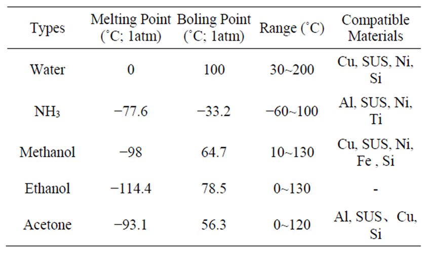
Table 1. Operating temperature of working fluid.
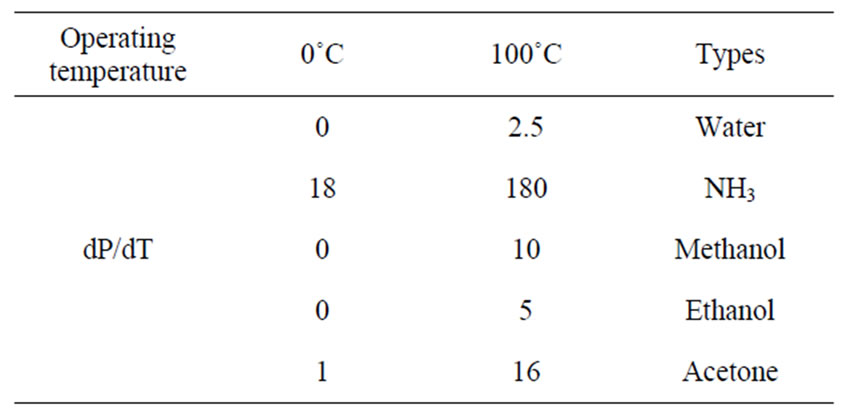
Table 2. Operating pressure of working fluid.
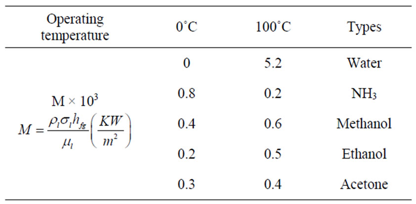
Table 3. Merit number of working fluid.
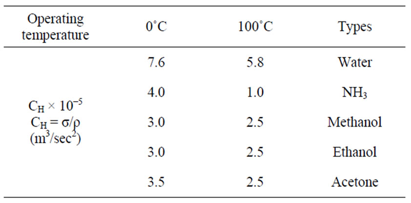
Table 4. Capillary parameter of working fluid.
2.2. Numerical Software
2.2.1. Introduction
This research uses CFD commercial software for the thermal and fluid analysis software “Thermal Desktop” of American C & R Technologies Corporation [16]. Its core processing program Sinda/Fluint was developed by the 1960s American outer-space planning program, “Cinda Code”. The first edition was established in 1986 by NASA. In 1992, the formal edition was officially published by C & R Corporation as the commercial version software. In this software, Sinda was used to compute the thermal resistances program; Fluint was designed to compute the flow resistance program. In 1991, after NASA officially adopted the heat flow analysis software of C & R Corporation, it obtained vital confirmation regarding outer-space science and technology in application. Sinda/Fluint also already had 40 years experience in the application of the US aerospace field. The software also once had the honor of receiving NASA’s contribution award in 1991. Therefore, the present country and organization in the world that participated in the NASA corporate plan must use Sinda/Fluint to carry on the thermal and fluid analysis design. After that, it would receive the affirmation in the fields of the automobile industry, air conditioning industry, American military, and aerospace industry.
2.2.2. Feature
This software utilizes the unique Finite Network Method (FNM). After the thermal and fluid problem has expressed its characteristics in a parallel network way, the computation is started in an in-series network way. This method can quickly and precisely compute the heat flow problem. The features of the software are as follows:
1) Sinda/Fluint is a set of the merit processing program which combines finite element method (FEM) and finite difference method (FDM). Unique FNM, which solves the heat transfer and flowing problem by the so-called equality solution law, quickly obtains the analysis exact solution of the thermal and fluid problem.
2) Sinda/Fluint only needs to establish the model of the thermal and fluid problem and can quickly and precisely simulate the physical problems of heat conduction, heat radiation, heat convection, two-phase flow, and refrigeration at low temperatures.
3) Sinda/Fluint is the most powerful thermal and fluid software in the field of design and analysis, and is often used in mechanical components, such as elbow, pipe acessories, pumps, ventilators and so on, which are subject to the parameters of the software. Unique FNM, which analyzes the interior phenomenon of the complex twophase flow, is especially powerful and practical.
4) Sinda/Fluint is the smartest thermal and fluid design software in the world today. The software commences without requiring all parameters. Also, it can get the system’s optimization from all parameters one designs. At the same time, it carries on the reliable analysis in the numerous variables assigned.
From the above features of this software, the present study uses the commercial software which is quite formidable. Furthermore, it calculates rapidly and precisely, and because it is the analysis software of the thermal and fluid project which NASA instigated, the results of the simulation analysis have strong, practical values indeed.
2.3. Analysis Method
This research first selects a set of experimental data with a power input of 3.3 W, a heat pipe effective thermal resistance of 1.28 ˚C/W, and a non-condensation gas of 1.43 × 10⁻¹³ g [15]. The procedure of the simulation analysis is as follows:
The first step was to use AutoCAD software of TD (Thermal Desktop) to draw the 3-D simulation model of the heat pipe, illustrated in Figure 2. Its size for the outer diameter is 3 mm, and the total length 200 mm. The second step was to utilize the attributions of the heat pipe in TD and designate Figure 2 as the heat pipe model with a wall thickness of 0.3 mm. The hypothesis grid element is 200. The third step was to establish the heat pipe internal simulation parameter. The heat pipe material is copper, the working fluid is the water, the heat transfer coefficient of the evaporation section is 0.00864 W/mm2K, the heat transfer coefficient of the condensation section is 0.13264 W/mm2K, and the mass of the non-condensation gas is 1.43 × 10⁻¹³ g. Then, to select the first 50 mm length of heat pipe is the heat source input, named evaporation section. The latter 50 mm length of heat pipe is the choice region for the cooling jacket input, called the condensation section, which sets the temperature at 33˚C. The fourth step was to set up the boundary and the steady-state condition. Lastly, was to carry on the solution and post-process of the demonstra tion of the flow field. After the first set of results from the simulation analysis and experimental data, the heat source power input was
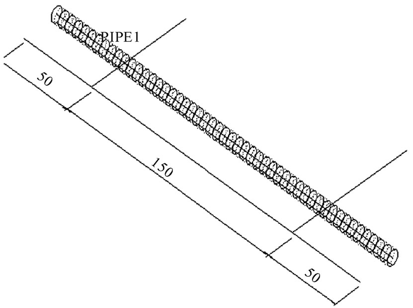
Figure 2. Single heat pipe model.
changed to 5.0 W and 6.5 W to start the solution. Each set of simulated time may obtain a precise analysis result in several minutes.
3. Results and Discussions
In view of the temperature-measured point of the simple heat pipe, the evaporation, adiabatic and condensation sections have different positions. The positions of the evaporation section were 16 mm and 32 mm, the positions of the adiabatic section were 83 mm and 116 mm and the positions of the condensation section were 160 mm, 175 mm and 190 mm. As shown in Figure 3, the temperature distributions of the simple heat pipe is at the power input of 3.3 W. The temperature of the evaporation section is between 42.4˚C and 43.1˚C, and of the condensation section 41.3˚C. When the power input is 3.3 W, the deviation between the simulation and the experiment is 4.4% for the evaporation section, 3.4% for the adiabatic section, and 3.1% for the condensation section. Figure 4 illustrates the temperature curves of the experiment and simulation at 3.3 W; the numerical results for the temperature of evaporation section are lower than the experimental data by 1.9˚C. The non-evaporation section has been 1.8˚C higher than the experimental value. This is because of the issues with the numerical simulation analysis in the parameter hypothesis difference, simulation heat source power input, cooling jacket’s fixed temperature, and mass of non-condensation gas to have an error with the actual value.
Figure 5 illustrates the temperature distributions of the simple heat pipe at a power input of 5 W. The temperature of the evaporation section is between 47.2˚C and 48.3˚C, and the temperature of the condensation section is 45.5˚C. When the power input is 5 W, the deviation between calculation and experiment is 3.55% for the evaporation section, 3.8% for the adiabatic section, and 3.4% for the condensation section. Figure 6 shows the temperature curves of the simulation and the experiment at 5 W. The numerical calculation is lower than the experimental value by 1.8˚C, and the non-evaporation section has a 1.7˚C higher value than the experiment. From these figures, the temperature profile tendency at a power input of 3.3 W and 5 W is consistent with the numerical result and the experimental data. This means that the numerical result in this study is correct.
Figure 7 depicts the temperature distributions of the single heat pipe at a power input of 6.5 W. The temperature of the evaporation section is between 51.4˚C and 52.9˚C. The temperature in the condensation section is 49.3˚C. When the power input is 6.5 W, the average error of the numerical and experimental results is 5.8% for the evaporation section, 6.7% for the adiabatic section, and 2.1% for the condensation section. The error has rea-
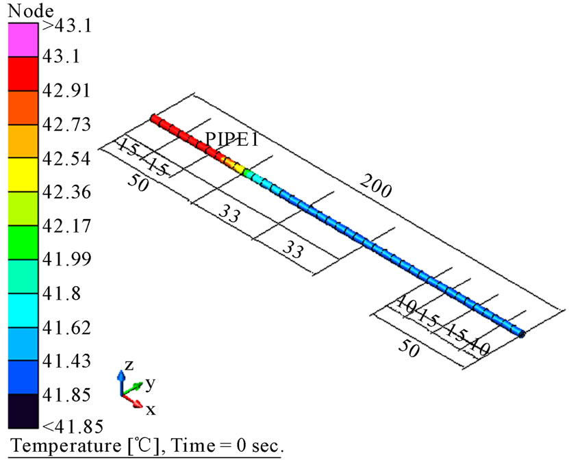
Figure 3. Heat pipe temperature of 3.3 Watt heater.
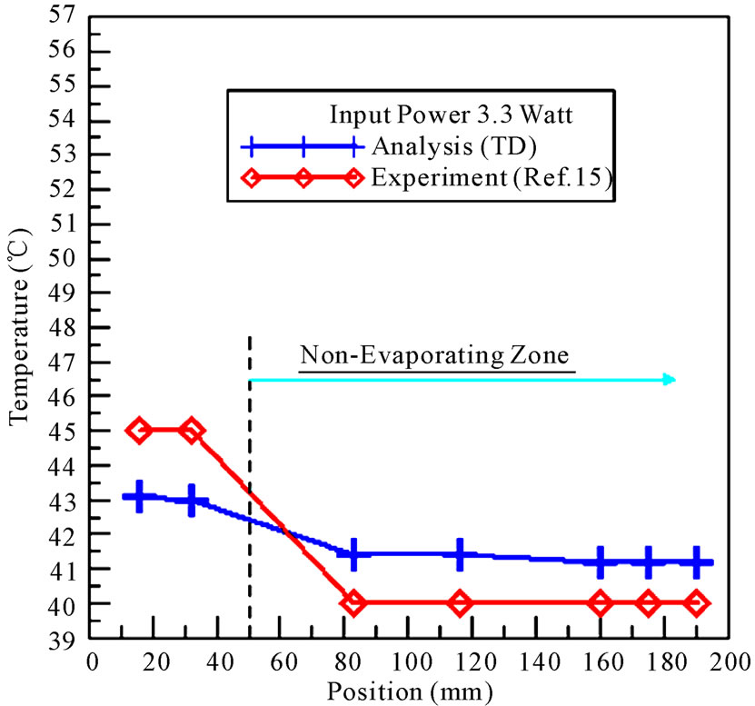
Figure 4. Temperature curves vs. thermal couple position for analysis and experiment of 3.3 Watt heater.
ched above 5% in the evaporation and adiabatic sections, compared to 3.3 W and a 5 W, but the error of the condensation section is quite small. The entire deviation of the slope is too large. This may have larger error measurement possibility in the experiment [15]. Figure 8 shows the temperature curve of the numerical result and the experiment data at 6.5 W. The numerical calculations of the evaporation and non-evaporation sections are lower than the experimental values by 3.1˚C and 2.5˚C, respectively. Comparing the temperature curve of the experimental data between Figures 5 and 6, the three temperatures in the non-evaporation section have higher values than in Figure 8, which caused the larger computational error. The reason is that the effect of the adiabatic section in the experiment is invalid and the other reason

Figure 5. Heat pipe temperature of 5.0 Watt heater.
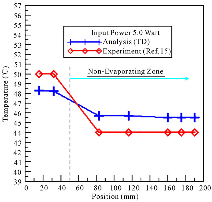
Figure 6. Temperature curves vs. thermal couple position for analysis and experiment of 5.0 Watt heater.
is that there is a difference between the mass of the noncondensation gas in the experiment and the input values of the parameters. This study suggests that the single heat pipe at 6.5 W in the experiments should be tested again.
In comparison of non-condensation gas to the thermal performance of the heat pipe, Figures 9-11 show the temperature distributions under the different percentages. When the non-condensation gas percentage is lower, the difference between the evaporation section and the condensation section is smaller. As the non-condensation gas percentage reaches as high as 0.01%, the mean temperature difference at both sides will be 12˚C higher. When the percentage reduces to 0.0001%, the temperature difference between the evaporation and condensa-
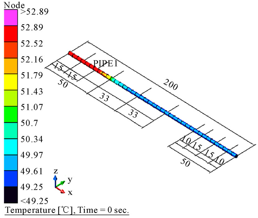
Figure 7. Heat pipe temperature of 6.5 Watt heater.
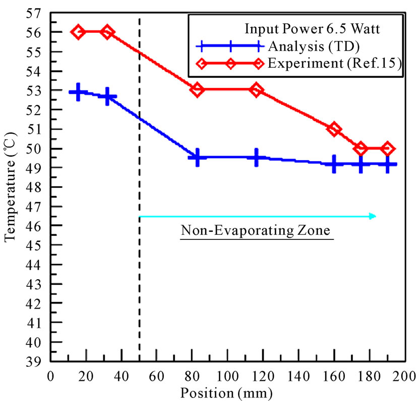
Figure 8. Temperature curves vs. thermal couple position for analysis and experiment of 6.5 Watt heater.
tion sections is below 3˚C. If the heat pipe interior does not completely have non-condensation gas, the temperature difference will be smaller than 0.1˚C. When the temperature difference of the evaporation section and the condensation section is reduced, the heat source temperature is also decreased. Therefore, the interior noncondensation gas in the heat pipe is smaller at the same power input, the heat source temperature is lower, and the thermal performance of the heat pipe is better. From Figure 12, when the non-condensation gas percentage is smaller than 0.00008%, the average temperature difference of both sides is already smaller than 1˚C, and the single heat pipe has reached its peak performance. At this stage, the heat pipe has the largest heat transfer rate.
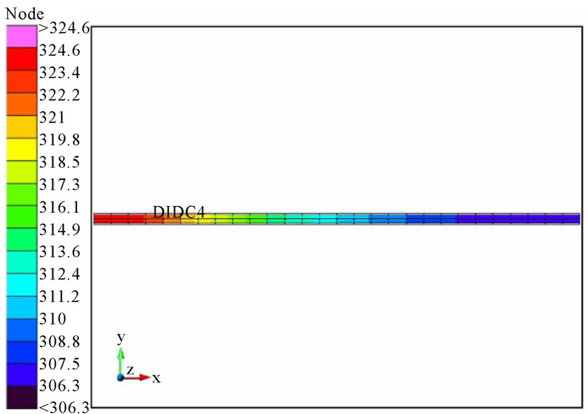
Figure 9. Heat pipe temperature of non-condensation gas 0.01%.

Figure 10. Heat pipe temperature of non-condensation gas 0.0001%.
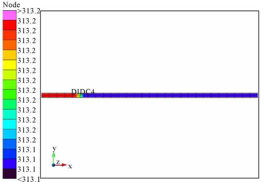
Figure 11. Heat pipe temperature of non-condensation gas 0.0%.
4. Conclusions
This research utilizes CFD software to simulate the thermal performance of a single heat pipe, and discusses the
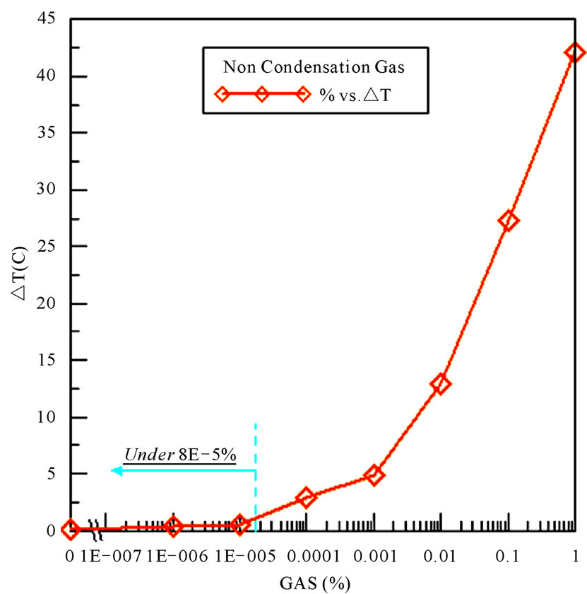
Figure 12. Heat pipe temperature difference vs. amount of non-conden-sation gas.
percentage of the non-condensation gas to influence the system. From the results, the deviation of the numerical result and the experimental data is below 6%. This means that this paper, which reported using the Thermal Desktop heat flow analysis special-purpose software to obtain the results, is sound. Therefore, when research and development manufacturers investigate the single heat pipe or the heat pipe module, these research results will be useful for the heat pipe industry as well as for academic reference.
5. Acknowledgements
The author thanks HyperInfo Company, Prof. Yu-Lieh Wu and all participants of the department of air condition and energy in the National Chin-Yi University of Technology in this research.
6. REFERENCES
- G. M. Grover, “US Patent No. 3229759,” 1963.
- G. P. Peterson, “An Introduction to Heat Pipe—Modeling, Testing, and Applications,” John Wiley & Sons Inc., New York, 1994.
- Y. Wang and G. P. Peterson, “Investigation of a Novel Flat Heat Pipe,” Journal of Heat Transfer, Vol. 127, No. 2, 2005, pp. 165-170. doi:10.1115/1.1842789
- A. Faghri, “Heat Pipe Science and Technology,” Taylor and Francis Ltd., Washington DC, 1995.
- V. G. Rajesha and K. P. Ravindrana, “Optimum Heat Pipe Design: A Nonlinear Programming Approach,” International Communications in Heat and Mass Transfer, Vol. 24, No. 3, 1997, pp. 371-380. doi:10.1016/S0735-1933(97)00022-5
- F. Lefevre and M. Lallemand, “Coupled Thermal and Hydrodynamic Models of Flat Micro Heat Pipes for the Cooling of Multiple Electronic Components,” International Journal of Heat and Mass Transfer, Vol. 49, No. 7-8, 2006, pp. 1375-1383. doi:10.1016/j.ijheatmasstransfer.2005.10.001
- G. P. Peterson and L. S. Fletcher, “Effective Thermal Conductivity of Sintered Heat Pipe Wicks,” Journal of Thermophysics, Vol. 1, No. 4, 1987, pp.343-347. doi:10.2514/3.50
- G. Mohamed, L. M. Hung and J. M. Tournier, “Transient Experiments of an Inclined Copper Water Heat Pipe,” Journal of Thermophysics and Heat Transfer, Vol. 9, No. 1, 1995, pp.109-116.
- X. L. Xie, Y. L. He, W. Q Tao and H. W. Yang, “An Experimental Investigation on a Novel High-Performance Integrated Heat Pipe—Heat Sink for High-Flux Chip Cooling,” Applied Thermal Engineering, Vol. 28, 2008, pp. 433-439. doi:10.1016/j.applthermaleng.2007.05.010
- D. A. Beson and C. V. Robino, “Design and Testing of Metal and Silicon Heat Spreaders with Embedded Micromachined Heat Pipes,” American Society of Mechanical Engineers, Vol. 26, 1999, pp. 2-8.
- N. J. Gernert, J. Toth and J. Hartenstine, “100 W/cm2 and Higher Heat Flux Dissipation Using Heat Pipes,” 13th International Heat Pipe Conference, 21-25 September 2004, Shanghai, pp. 256-262.
- J.-C. Wang, “Superposition Method to Investigate the Thermal Performance of Heat Sink with Embedded Heat Pipes,” International Communication in Heat and Mass Transfer, Vol. 36, No. 7, 2009, pp. 686-692. doi:10.1016/j.icheatmasstransfer.2009.04.008
- J.-C. Wang, R.-T. Wang, C.-C. Chang and C.-L. Huang, “Program for Rapid Computation of the Thermal Performance of a Heat Sink with Embedded Heat Pipes,” Journal of the Chinese Society of Mechanical Engineers, Vol. 31, No. 1, 2010, pp. 21-28.
- J.-C. Wang, “L-Type Heat Pipes Application in Electronic Cooling System,” International Journal of Thermal Sciences, Vol. 50, No. 1, 2011, pp.97-105. doi:10.1016/j.ijthermalsci.2010.07.001
- W. H. Huang, “Fabrication and Performance Testing of Sintered Miniature Heat Pipe,” M. E. Master Thesis, National Taiwan University, Taiwan, 2000.
- 20 December 2010. http://www.crtech.com/