Intelligent Control and Automation
Vol. 3 No. 2 (2012) , Article ID: 19245 , 9 pages DOI:10.4236/ica.2012.32021
The Bezier Control Points Method for Solving Delay Differential Equation
Department of Applied Mathematics, Ferdowsi University of Mashhad, Mashhad, Iran
Email: fatemeghomanjani@gmail.com, farahi@math.um.ac.ir
Received December 19, 2011; revised January 30, 2012; accepted February 9, 2012
Keywords: Bezier Control Points; Delay Differential Equation; Residual Function; Boundary Value Problem; Proportional Delays
ABSTRACT
In this paper, Bezier surface form is used to find the approximate solution of delay differential equations (DDE’s). By using a recurrence relation and the traditional least square minimization method, the best control points of residual function can be found where those control points determine the approximate solution of DDE. Some examples are given to show efficiency of the proposed method.
1. Introduction
Delay differential equations are type of differential equations where the time derivatives at the current time depend on the solution, and possibly its derivatives, at previous times. A class of such equations, which involve derivatives with delays as well as the solution itself has been called neutral DDEs over the past century (see [1, 2]).
The basic theory concerning the stable factors and works on fundamental theory, e.g., existence and uniqueness of solutions, was presented in [1,2]. Since then, DDE have been extensively studied in recent decades and a great number of monographs have been published including significant works on dynamics of DDEs by Hale and Lunel [3], on stability by Niculescu [4], and so on. The interest in study of DDEs is caused by the fact that many processes have time-delays and have been models for better representations by systems of DDEs in science, engineering, economics, etc. Such systems, however, are still not feasible to actively analyze and control precisely, thus, the study of systems of DDEs has actively been conducted over the recent decades (see [1, 2]).
In this paper, we show a novel strategy by using the Bezier curves to find the approximate solution for delay differential equations by Bezier curves. Other numerical methods for DDEs are available in (see [5-8]). In section 2 delay differential equations will be introduced. Example of Time-Delay System will be stated in section 3. In section 4 delay differential equations with proportional delay will be introduced. Bezier curves and degree elevation will be stated in Sections 5 and 6 respectively. In Section 7 solution of delay differential equation using Bezier control points presented and aforementioned method will be implemented on it. In section 8, solved numerical examples, showed the efficiency and reliability of the method. Finally, section 9 will give a conclusion briefly.
2. Delay Differential Equations
Most delay differential equations that arise in population dynamics and epidemiology model intrinsically nonnegative quantities. Therefore it is important to establish that nonnegative initial data give rise to nonnegative solutions. Consider the following
 (2.1)
(2.1)
with a single delay h > 0. Assume that  and
and  are continuous on R3. Let
  be given and let
  be continuous. We seek a solution
  of (2.1) satisfying
 (2.2)
(2.2)
and satisfying (2.1) on  for some
 . Note that we must interpret
  as the right-hand derivative at s.
Now, we present a typical example of physical systems that exhibit time-delay phenomena. The example selected in this section fit nicely into the model (2.1).
3. Example of Time-Delay System
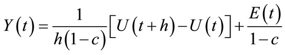
The existence of delays (or gestation lags) in economic systems is quite natural since there must be finite period of time following a decision for its effects to appear. In one model [9] of aggregate economy, we let  be the income which can split into consumption
 , investment
  and autonomous expenditure.
Thus
 (3.1)
(3.1)
Define
 (3.2)
(3.2)
where c is a consumption coefficient. From (3.1) we get
 (3.3)
(3.3)
It is assumed that there is finite interval of time between ordering and delivery of capital equipment following a decision to invest  In terms of the stock of capital assets
  we have
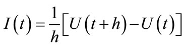
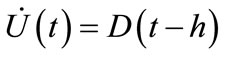 (3.4)
(3.4)
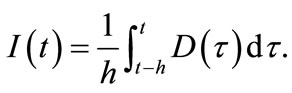 (3.5)
(3.5)
Economic rationale implies that  is determined by the rate of saving (proportional to
 ) and by the capital stock
 . This means that
 (3.6)
(3.6)
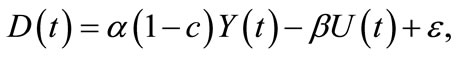
where ,
,  and ε is a trend factor. Combining (3.4) and (3.5), we obtain:
 (3.7)
(3.7)
By (3.3) and (3.7), we arrive at
 (3.8)
(3.8)
Finally, it follows from (3.5), (3.6) and (3.8) that
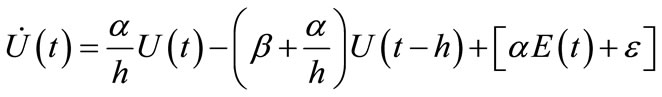 (3.9)
(3.9)
which expresses the formation of the rate of delivery of the new equipment. This is a typical functional differential equation (FDE) of retarded type.
4. Delay Differential Equations with Proportional Delay
In this paper, approximate analytical solutions with high accuracy can be obtained by carrying out in the Bezier control points method.
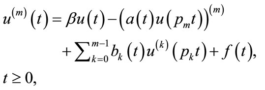
Consider the following neutral functional-differential equation with proportional delays (see [10-12]),
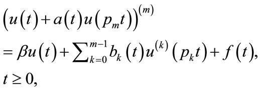 (4.1)
(4.1)
with the initial conditions
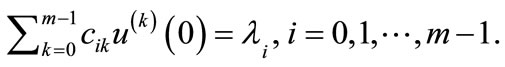 (4.2)
(4.2)
Here,  and
and  are given analytical functions, and
 ,
,  ,
,  ,
,  denote given constants with
The existence and the uniqueness of the analytic solution of the multi-pantograph equation are proved in [13], the Dirichlet series solution is constructed, and the sufficient condition of the asymptotic stability for the analytic solution is obtained. It is proved that the θ-methods with a variable stepsize are asymptotically stable if 
Some numerical examples are given to show the properties of the θ-methods.
In order to apply the Bezier control points method, we rewrite Equation (4.1) as
Neutral functional-differential equations with proportional delays represent a particular class of delay differential equation. Such functional-differential equations play an important role in the mathematical modeling of real world phenomena [14]. Obviously, most of these equations cannot be solved exactly. It is therefore necessary to design efficient numerical methods to approximate their solutions. Ishiwata et al. used the rational approximation method [15] and the collocation method [16] to compute numerical solutions of delay differential equations with proportional delays. Hu et al. [17] applied linear multistep methods to compute numerical solutions for neutral delay differential equations. Wang et al. obtained approximate solutions for neutral delay differential equations by continuous Runge-Kutta methods [18] and oneleg θ-methods [13,19].
5. Bezier Curves
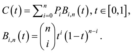
A Bezier curve of degree n can be defined as follows (see [19]):
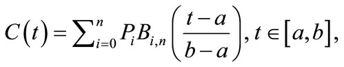 (5.1)
(5.1)
where 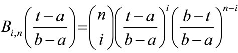 are the Bernstein polynomials over the interval
 . The Bezier coefficient
  is called the control point (see Figure 1). In particular
 (5.2)
(5.2)
If  be a vector-valued polynomial, then
  is called a parametric Bezier curve. The control polygon of a Bezier curve comprise of the line segments
 . If
. If  is a scalar-valued polynomial, we call the function
  an explicit Bezier curve by
  (see [20,21]).
6. Degree Elevation
Suppose we were designing with Bezier curve as described, and use a Bezier polygon of degree n to approximate the desired given shape. Suppose the degree polygon dose not feat neatly the desired shape.
One way to proceed in such a situation is to increase the flexibility of the polygon by adding another vertex (control point) to it. As a first step, one might want to add another vertex, yet leave the desired curve of the shape unchanged, this corresponds to raising the degree of the Bezier curve by one (see Figure 2). Therefore, we are looking for a curve with control vertices  that describes the same curve of the shape as the original polygon
  (see [21-25] for more details).
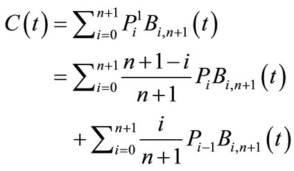
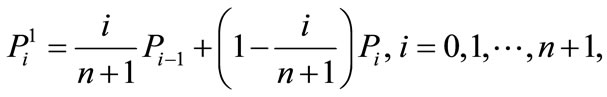
We rewrite our given Bezier curve as
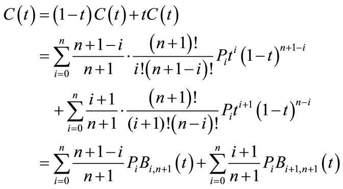
The upper index of the first sum may be extended to n + 1, since the corresponding term is zero. The summation indices of the second sum may be shifted to index 1 and n + 1, but one may choose the lower index zero since only a zero term is added. Thus we have
 (6.1)
(6.1)
Combining both sums and computing coefficients
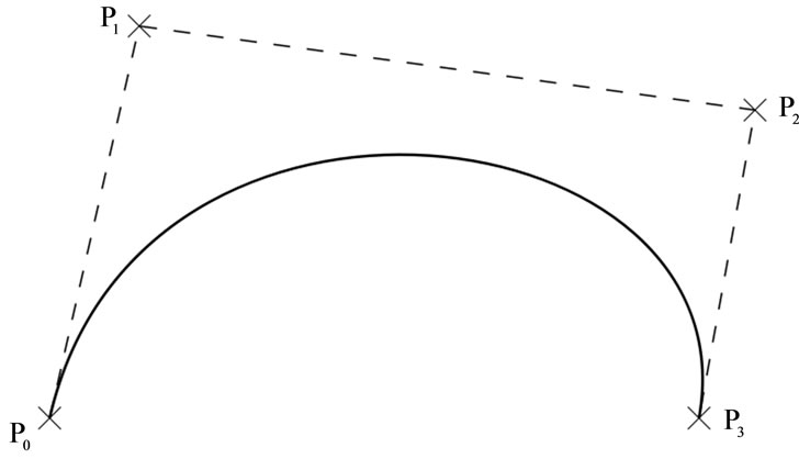
Figure 1. A degree three Bezier curve and its control polygon.
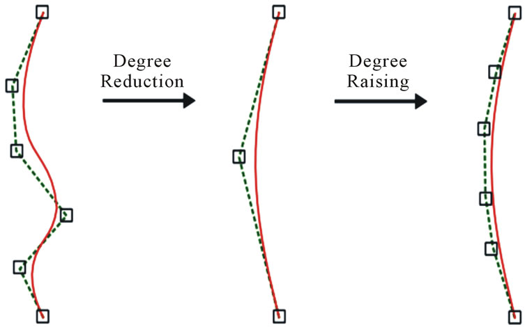
Figure 2. Repeated degree elevation.
yields:
 (6.2)
(6.2)
where  is the control point of the Bezier curve
  when it is elevated to degree n + 1. Now, the new control polygon consists of n + 2 control points.
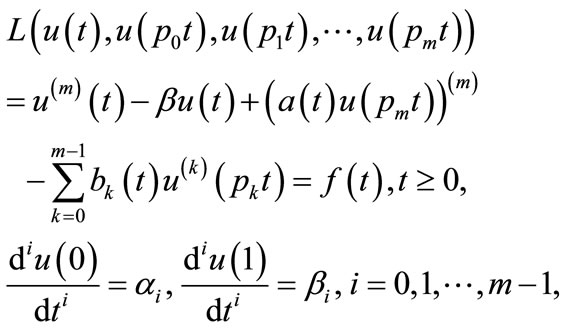
7. Solution of Delay Differential Equation Using Bezier Control Points
Consider the following boundary value problem
 (7.1)
(7.1)
where L is differential operator with proportional delay,  is also a polynomial in t, and
  (k = 0, 1, ··· , m) [26].
We propose to represent the approximate solution of (7.1)  in Bezier form. The choice of the Bezier form rather than the B-spline form is due to the fact that the Bezier form is easier to symbolically carry out the operations of multiplication, comparison and degree elevation than B-spline form. We choose the sum of squares of the Bezier control points of the residual to be the measure quantity. Minimizing this quantity gives the approximate solution. So, the obvious spotlight is in the following, if the minimizing of the quantity is zero, so the residual function is zero, which implies that the solution is the exact solution. We call this approach the control-point-based method. The detailed steps of the method are as follows (see [24]):
• Step 1. Choose a degree n and symbolically express the solution  in the degree
  Bezier form
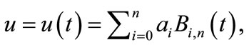 (7.2)
(7.2)
where the control points  are to be determined.
• Step 2. Substituting the approximate solution  into the differential Equation (7.1), we gain the residual function

This is a polynomial in t with degree ≤ k, where
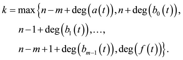
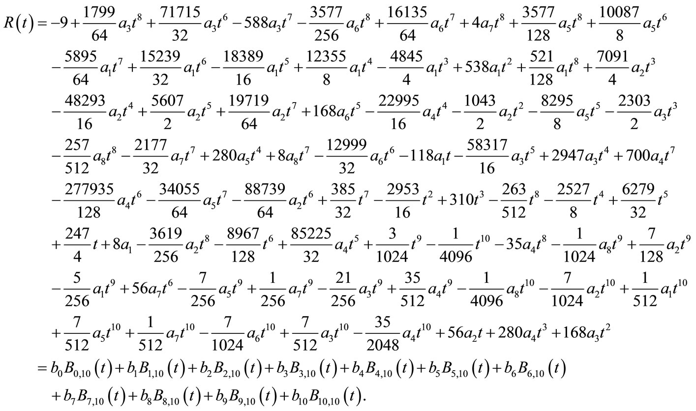
So the residual function  can be expressed in Bezier form as well,
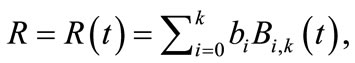 (7.3)
(7.3)
where the control points  are linear functions in the unknowns
 . These functions are derived using the operations of multiplication, degree elevation and differentiation for Bezier form.
• Step 3. Construct the objective function  Then F is also a function of
 .
.
• Step 4. Solve the constrained optimization problem:
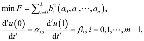 (7.4)
(7.4)
by some optimization techniques, such as Lagrange multipliers method, we can be used to solve (7.4).
• Step 5. Substituting the minimum solution back into (7.2) arrives at the approximate solution to the differential equation.
8. Numerical Examples
In this part, we used the mentioned control-point-based method on Bezier control points to solve DDE’s and system of DDE’s.
Example 8.1. As a practical example, we consider Evens and Raslan [6] the following pantograph delay equation:
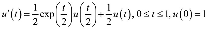 .
.
The exact solution is . Now we try to find a degree two approximate solution. Let
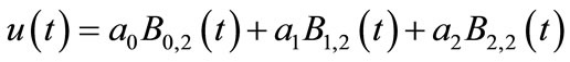 .
.
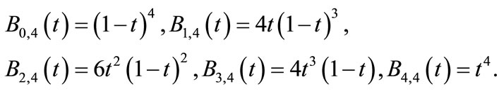
Substituting it into the above delay differential equation gives  as:
as:
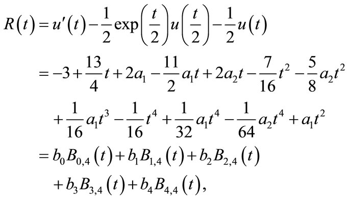
where
Then construct the function
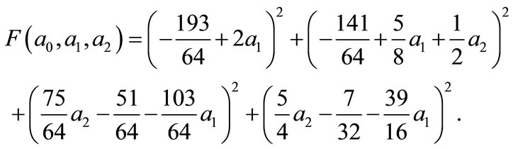
Minimizing  with
with  and u(1) = a2 = exp(1). We obtain
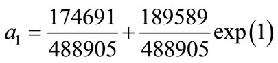 .
.
Thus the approximate solution is
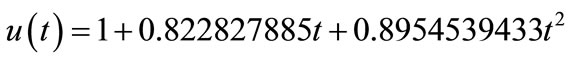 .
.
In Figure 3 compare approximated and exact value of . Figure 4 shows the residual function.
Example 8.2. Consider the previous example with degree raising in Bezier control points.
Let

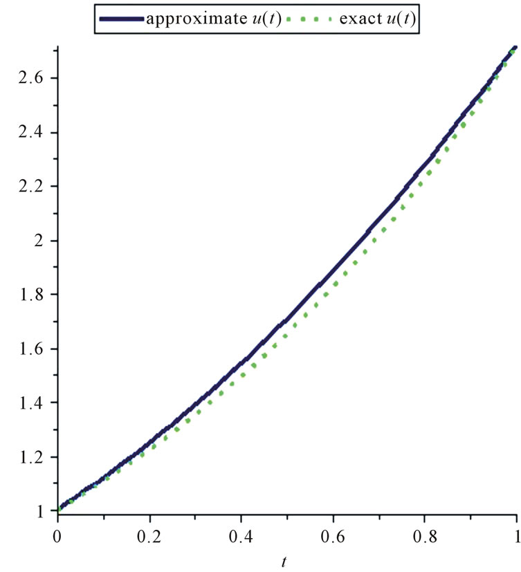
Figure 3. Approximate and exact solution of u(t) for Example 8.1.

Figure 4. Residual function for Example 8.1.
Substituting it into the delay differential equation leads to  as:
as:
Then construct the function
and minimizing F with  and u(1) = a8 = exp(1). We obtain

and
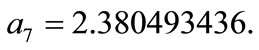
Thus the approximate solution is
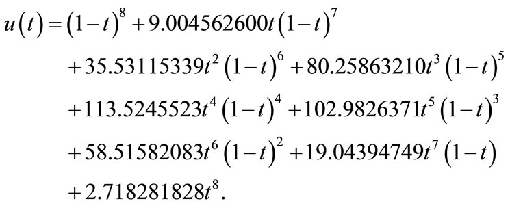
In Figure 5 compare approximated and exact value of . Figure 6 shows the residual function.
Figure 5. Approximate and exact solution of u(t) for Example 8.2.
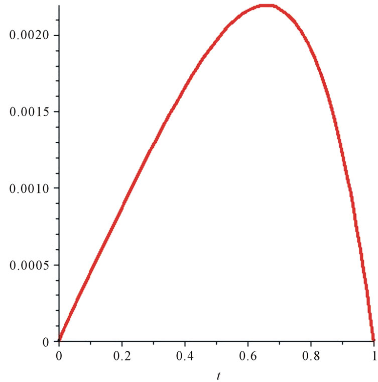
Figure 6. Residual function for Example 8.2.
Example 8.3. Consider the following second order linear DDE (see [5]):
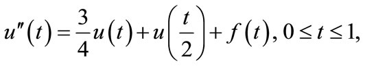
where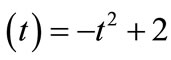 , with initial conditions
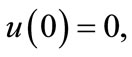
 , and the exact solution is
 .
.
Let
By applying this algorithm, we obtain 


and . Thus the approximate solution is
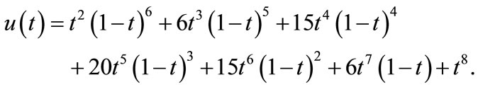
Figure 7, compares the exact and approximate solution of . Figure 8 shows the residual function.
Example 8.4. Consider the following second order linear DDE (see [10]):
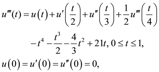
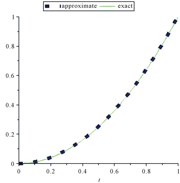
Figure 7. Approximate and exact solution u(t) for Example 8.3.
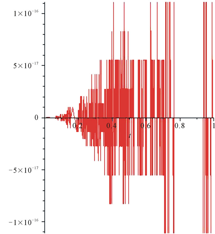
Figure 8. Residual function for Example 8.3.
where the exact solution is . Let
. Let

By applying this algorithm, we obtain 


and . Thus the approximate solution is
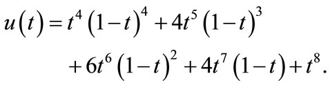
Figure 9, compares the exact and approximate solution of . Figure 10 shows the residual function.
Example 8.5. In this example the following first order linear DDE’s is considered (see [13]):
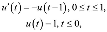
Since  and
and ,
,  has a jump at t = 0. The second derivative
and therefore it has a jump at t = 1.
Now we try to find an approximate solution. Let
 .
.
By applying this algorithm, we acquire ,
,  ,
,  ,
, . Thus
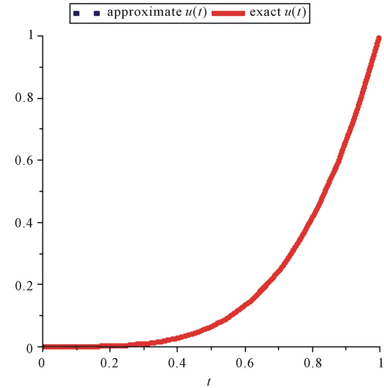
Figure 9. Approximate and exact solution u(t) for Example 8.4.
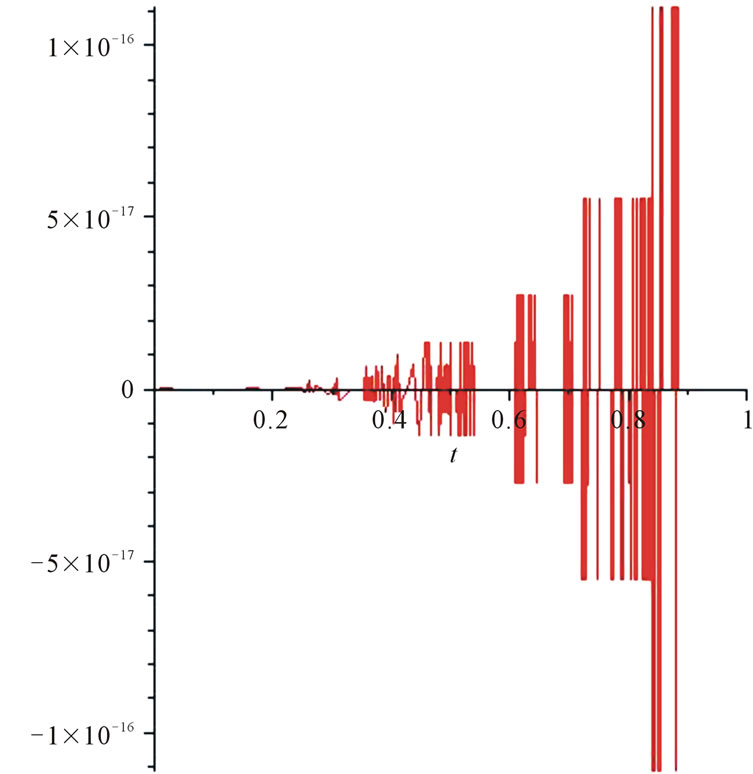
Figure 10. Residual function for Example 8.4.
the approximate solution is
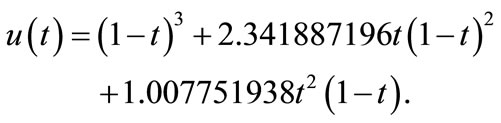
Figure 11 shows the approximate value of .
.
9. Conclusion
In this paper, we use the control-point-based method to solve delay differential equations. In this method, firstly,
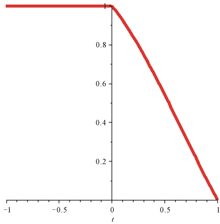
Figure 11. Approximate u(t) for Example 8.5.
the rough solution is expressed in Bezier form, then the residual function is minimized to find the best approximate solution. Some examples are given to verify the reliability and efficiency of the proposed method.
REFERENCES
- G. Adomian and R. Rach, “Nonlinear Stochastic Differential Delay Equation,” Journal of Mathematical Analysis and Applications, Vol. 91, No. 1, 1983, pp. 94-101. doi:10.1016/0022-247X(83)90094-X
- F. M. Asl and A. G. Ulsoy, “Analysis of a system of linear Delay Differential Equations,” Journal of Dynamic Systems, Measurement and Control, Vol. 125, No. 2, 2003, pp. 215-223. doi:10.1115/1.1568121
- J. K. Hale and S. M. V. Lunel, “Introduction to Functional Differential Equations,” Springer-Verlag, Berlin, 1993.
- S. I. Niculescu, “Delay Effects on Stability: a Robust Control Approach,” Springer, Berlin, 2001.
- A. K. Alomari, M. S. M. Noorani and R. Nazar, “Solution of Delay Differential Equation by means of Homotopy Analysis Method,” Acta Applicandae Mathematicae, Vol. 108, No. 2, 2009, pp. 395-412. doi:10.1007/s10440-008-9318-z
- D. J. Evans and K. R. Raslan, “The Adomian Decomposition Method for Solving Delay Differential Equation,” International Journal of Computer Mathematics, Vol. 82, No. 1, 2005, pp. 49-54. doi:10.1080/00207160412331286815
- S. J. Liao, “Series solutions of Unsteady Boundary-Layer Flows over plate,” Mathematical Analysis and Applications, Vol. 117, No. 3, 2006, pp. 239-263. doi:10.1111/j.1467-9590.2006.00354.x
- F. Shakeri and M. Dehghan, “Solution of Delay Diffrential Equation via a Homotopy Perturbation Method,” Mathematical and Computer Modelling, Vol. 48, No. 3-4, 2008, pp. 486-498. doi:10.1016/j.mcm.2007.09.016
- H. Gorecki, S. Fuksa, P. Grabowski and A. Korytowski, “Analysis and Synthesis of Time Delay Systems,” John Wiley and Sons, New York, 1989.
- X. Chen and L. Wang, “The Variational Iteration Method for solving a Neutral Functional-Differential Equation with Proportional Delays,” Computers and Mathematics with Applications, Vol. 59, No. 8, 2010, pp. 2696-2702. doi:10.1016/j.camwa.2010.01.037
- Z. Fan, M. Liu and W. Cao, “Existence and uniqueness of the solutions and convergence of Semi-Implicit Euler methods for Stochastic Pantograph Equations,” Mathematical Analysis and Applications, Vol. 325, No. 2, 2007, pp. 1142-1159. doi:10.1016/j.jmaa.2006.02.063
- R. Bellman and K. L. Cooke, “Differential-Difference Equations,” Academic press, London, 1963.
- W. Wang, T. Qin and S. Li, “Stability of One-Leg θ- methods for Nonlinear Neutral Differential Equations with Proportional Delay,” Applied Mathematics and Computation, Vol. 213, No. 1, 2009, pp. 177-183. doi:10.1016/j.amc.2009.03.010
- A. Bellen and M. Zennaro, “A reviw of DDE methods,” in: G. H. Golub, C. H. Schwab, W. A. Light and E. Suli, Eds., Numerical methods for Delay Differential Equations, Numerical Mathematics and Scientific Computation, Clarendon Press, New York, 2003, pp. 36-60.
- E. Ishiwata and Y. Muroya, “Rational Approximation Method for Delay Differential Equations with Proportional Delay,” Applied Mathematics and Computation, Vol. 187, No. 2, 2007, pp. 741-747. doi:10.1016/j.amc.2006.08.086
- E. Ishiwata, Y. Muroya and H. Brunner, “A Super-Attainable Order in Collocation Methods for Differential Equations with Proportional Delay,” Applied Mathematics and Computation, Vol. 198, No. 1, 2008, pp. 227-236. doi:10.1016/j.amc.2007.08.078
- P. Hu, C. Huang and S. Wu, “Asymptotic stability of Linear Multistep Methods for Nonlinear Neutral Delay Differential Equations,” Applied Mathematics and Computation, Vol. 211, No. 1, 2009, pp. 95-101. doi:10.1016/j.amc.2009.01.028
- W. Wang, Y. Zhang and S. Li, “Stability of continuous Runge-Kutta-Type Methods for Nonlinear Neutral DelayDifferential Equations,” Applied Mathematical Modelling, Vol. 33, No. 8, 2009, pp. 3319-3329. doi:10.1016/j.apm.2008.10.038
- W. Wang and S. Li, “On the One-Leg θ-methods for Solving Nonlinear Neutral Functional Differential Equations,” Applied Mathematics and Computation, Vol. 193, No. 1, 2007, pp. 285-301. doi:10.1016/j.amc.2007.03.064
- G. Farin, “Curves and surfaces for CAGO: A Practical Guide,” Morgan Kaufmann, Waltham, 2001.
- G. Farin, “Curves and surfaces for Computer-Aided geometric Design: A Practical Guide,” 4th edition, Academic press, London, 1997.
- S. Mann, “A Blossoming Development of spliness,” Morgan claypool, San Rafael, 2004.
- S. Biswa and B. Lovell, “Bezier and splines in image processing and Machine Vision,” springer-verlag, Berlin, 2008.
- J. Zheng, T. Sedberg and R. Johansons, “Least Squares Methods for Solving Differential Equation Using Bezier Control Points,” Applied Numerical Mathematics, Vol. 48, No. 2, 2004, pp. 137-152. doi:10.1016/j.apnum.2002.01.001
- B. Egerstedt and F. Martin, “A note on the connection between Bezier curves and Linear Optimal Control,” IEEE Transactions on Automatic Control, Vol. 49, No. 10, 2004, pp. 1728-1731. doi:10.1109/TAC.2004.835393
- M. Mahmoud and P. Shi, “Methodologies for control of Jump Time-Delay Systems,” Kluwer Academic publishers, London, 2004.