Materials Sciences and Applications
Vol.10 No.03(2019), Article ID:91512,40 pages
10.4236/msa.2019.103021
Oxidation Kinetics of Aluminum Powders in a Gas Fluidized Bed Reactor in the Potential Application of Surge Arresting Materials
Hong Shih
Etch Products Group, Lam Research Corporation, Fremont, CA, USA
![]()
Copyright © 2019 by author(s) and Scientific Research Publishing Inc.
This work is licensed under the Creative Commons Attribution International License (CC BY 4.0).
http://creativecommons.org/licenses/by/4.0/


Received: January 15, 2019; Accepted: March 26, 2019; Published: March 29, 2019
ABSTRACT
In this technical paper, the oxidation mechanism and kinetics of aluminum powders are discussed in great details. The potential applications of spherical aluminum powders after oxidation to be part of the surging arresting materials are discussed. Theoretical calculations of oxidation of spherical aluminum powders in a typical gas fluidization bed are demonstrated. Computer software written by the author is used to carry out the basic calculations of important parameters of a gas fluidization bed at different temperatures. A mathematical model of the dynamic system in a gas fluidization bed is developed and the analytical solution is obtained. The mathematical model can be used to estimate aluminum oxide thickness at a defined temperature. The mathematical model created in this study is evaluated and confirmed consistently with the experimental results on a gas fluidization bed. Detail technical discussion of the oxidation mechanism of aluminum is carried out. The mathematical deviations of the mathematical modeling have demonstrated in great details. This mathematical model developed in this study and validated with experimental results can bring a great value for the quantitative analysis of a gas fluidization bed in general from a theoretical point of view. It can be applied for the oxidation not only for aluminum spherical powders, but also for other spherical metal powders. The mathematical model developed can further enhance the applications of gas fluidization technology. In addition to the development of mathematical modeling of a gas fluidization bed reactor, the formation of oxide film through diffusion on both planar and spherical aluminum surfaces is analyzed through a thorough mathematical deviation using diffusion theory and Laplace transformation. The dominant defects and their impact to oxidation of aluminum are also discussed in detail. The well-controlled oxidation film on spherical metal powders such as aluminum and other metal spherical powders can potentially become an important part of switch devices of surge arresting materials, in general.
Keywords:
Aluminum, Spherical Power, Gas Fluidization Bed, Oxidation Mechanism, Oxide Growth Rate, Gibbs Free Energy, Ellingham Diagram, Mathematical Modeling, Dynamic System, Plasma, Diffusion, Diffusion Coefficient, Crystallographic Defect, Vacancy, Pressure, Temperature, Flow, Laplace Transform, Equation, Boundary Condition, Fick’s Second Law, Software, Experimental, Theoretical, Surge Arresting Materials, Analytical Solution

1. Introduction
Oxidation of aluminum to form aluminum oxide film has been playing significant roles in modern industry and receiving wide applications. Aluminum hard anodization has been widely using in semiconductor industry as chamber surface coating. The anodized aluminum through different oxidizing processes at low temperature in acidic solutions has demonstrated excellent performance in corrosion resistance for semiconductor plasma etching equipment from 200 mm silicon wafer fabrication to current 300 mm silicon wafer fabrication worldwide [1] - [28] . The high corrosion resistance, production repeatability, and low cost of anodized aluminum to form a unique oxide layer on aluminum alloys in acidic solutions have been widely used in semiconductor IC industry. Shih summarized the chamber materials performance for plasma etching chamber including anodized aluminum in his article [1] . Many technical papers have been published in the study of anodized aluminum and its applications [1] - [28] . The formation of oxide layer through logarithmic, parabolic, linear, and combinations of reaction rate in gas phases and the reaction mechanism of aluminum oxide formation described by many authors [29] - [42] . Aluminum powders can form a very thin oxide film in gas phases. Aluminum powders with a very thin oxide film may serve as switch material or called surge arresting materials (SAMs) when the aluminum powders with thin oxide layer and filler mix together. SAMs are electronic composite materials consisting of insulatively coated conductive and semiconductive particles which are embedded in a polymer binder or ceramic matrix. The calculation of ratio of mixing of aluminum powders and filler is based on the percolation theory [43] [44] [45] [46] [47] . From the percolation theory and the so-called “quantum mechanical tunneling”, SAMs can serve as switches which can pass voltage or current at a sufficiently high electric field. It means that the oxide film on aluminum powders can serve as a controller to switch on or switch off at a critical voltage or current. This application may bring a great interest for people to create a passive switch material in SAMs study.
As an n-type of semiconductor, aluminum oxide (Al2O3), is a metal excess oxide. The oxidation mechanism and the formation of metal oxide on metal surface at high temperature are summarized by Jones in his book [29] . Aluminum oxide has a Pilling Bedworth Ratio (PBR) as of 1.28 which is defined by the ratio of the molar volume of the oxide per gram atom to volume consumption of metal (Vox/Vmetal) [30] . According to PBR, the oxide will fail to cover the entire metal surface and will be non-protective when PBR is less than 1.0. The oxide will be protective when PBR is larger than 1.0. But PBR principally has a very limited application [31] and is only one of many factors which can determine the protective properties of an oxide film on metal. In the case of aluminum, the density of Al2O3 is less than aluminum metal, the oxide layer can cover the entire surface of aluminum, and the aluminum oxide is very protective. Typical PRB and the properties of metal oxides are summarized in Table 1 [29] as shown below.
Ellingham diagram has been used to show the relationship of Gibbs free energy versus temperature for oxidation of metals [32] [33] [34] .
In order to make the oxide film on metals as switch material, one has to control the growth rate and the uniformity of the oxide film on metals very well. It means that the thickness of oxide on metals and the uniformity of thickness of oxide layer have to be controlled very well during oxidation. The major properties are the thickness of oxide layer and the uniformity of the oxide film. Taking consideration of aluminum powder oxidation, the selection of aluminum powders and the methodology to form the aluminum oxide film are very important.

Table 1. Properties of metal oxides.
P: Protective; NP: Not Protective; n: n-type semiconductor, metal excess oxide; p: p-type semiconductor, metal deficit oxide from Jones [29] .
The spherical shape of aluminum powders in a gas phase fluidized bed can help to produce a uniform aluminum oxide film. A fluidized bed has been used for gas and solid particles interaction for many years. The term FLUIDIZATION is used to designate the gas-solid contacting process in which a bed of finely divided solid particles is lifted and agitated by a rising stream of process gas. At the lower end of the velocity range, the amount of lifting is slight, the bed behaving likes a boiling liquid. At the other extreme, the particles are fully suspended in the gas stream and are carried along with it. The terms of suspension, suspensoid, and entrainment contact have all been used to designate this action.
The fluidized technique was born from the pioneering work of Standard Oil Development Company and was introduced commercially in 1937. The development of the technique was summarized by Zenz [48] . During the past succeeding years, the application of the fluidization technology has spread rapidly to metallurgical ore roasting, limestone calcination, synthetic gasoline, petrochemicals, nuclear reactors, corrosion resistance materials, as well as surge arresting materials. There are many advantages of the fluidized technique. The advantages are listed as below:
1) Excellent temperature control to reach isothermal conditions.
2) Continuity of operation.
3) Heat transfer.
4) Catalytic gas reactions.
5) Aeratable powders have the most desirable fluidization properties.
6) Interparticle forces in the particles are significantly smaller than hydrodynamic forces and gas bubbles are limited in size.
The heat transfer, minimum fluidization velocity, fluidization technology, and packing properties have been discussed by various authors [49] - [54] . In order to operate the fluidized bed in bubble conditions and to avoid the occurrence of slugging, channeling, jetting, and spouting, the experimental design is very important. Many factors are involved in this technique. The bubble formation and types of fluidization are shown in Figure 1 and Figure 2, respectively.
Although gas fluidization bed has been using in different applications for many years, there is no theoretical modeling available. It means that the oxide formation relies on experimental results. The author needs to develop the theoretical model based on the dynamic system with specific hydrodynamic flow conditions. The current work is to create and to build up a theoretical mathematic modeling based on the real dynamic system and system parameters to estimate the thickness of oxide layer in a gas fluidization bed. Therefore, one can carry on the theoretical calculation and compare the results with experiments. In fact, the mathematical model developed in this work can help to carry out quantitative calculation of oxide growth rate at different conditions and compare the calculation with experimental results. Taking aluminum ball powder as an example, the author successfully created and developed the mathematical modeling and applied the model to compare with experimental results on a gas fluidization bed [55] - [60] .

Figure 1. Bubble formation from bed-penetrating gas jets at the grit points.

Figure 2. Types of fluidization.
2. Theoretical Calculation of a Gas Fluidization Bed Reactor (FBR)
1) Basic parameters used in the kinetic calculation of a gas fluidization bed reactor:
π = 3.1416.
Ssur = πD2 = surface area of aluminum ball with diameter, D.
Din = Inner diameter of bed = 70 mm = 7.0 cm = 0.070 m.
Dout = Outer diameter of bed = 75 mm = 7.5 cm = 0.075 m.
Bed wall thickness = 2.5 mm = 0.25 cm = 0.0025 m.
Area of cross section of bed = = 38.48 cm2.
Height of bed = 9.0 inch = 229.4 mm = 22.94 cm = 0.229 m.
Total volume of bed = 883 cm3.
Material of fluidization bed is quartz.
Thickness of the gas distributor = 5 mm = 0.5 cm = 0.005 m.
Hole size of the gas distributor = 10 μm - 15 μm.
Number of holes on the gas distributor ≈ 1000.
2) Parameters and bed operation conditions:
Volume flow rate of dry air = 8.333 × 10⁻⁵ m3/sec = 83.33 cm3/sec.
Weight of aluminum powders = 1.5 pounds.
Average diameter of aluminum powders = 20.0 μm.
The velocity of dry air = 2.16 cm/sec.
The height of air flowing = 130.3 cm/min.
Particle size distribution of aluminum powder is between 10 μm and 100 μm.
Temperature is between 25˚C and 400˚C.
Density of aluminum particles = 2700 kg/m3.
Bed bulk density = 1.414 kg/m3.
Bed void before fluidization = 0.4764.
Thermal conductivity of air at 100˚C = 0.0286 W·m−1·K−1.
Thermal conductivity of air at 200˚C = 0.0370 W·m−1·K−1.
Specific heat of quartz = 0.80 kJ·kg−1·K−1.
Specific heat of air = 1.03 kJ·kg−1·K−1.
Specific heat of aluminum powders = 0.982 kJ·kg−1·K−1.
Air flow rate in kg/sec. = 5.80 × 10⁻⁵ kg/sec.
Density of air at 200˚C = 0.696 kg/m3.
Density of air at 100˚C = 0.927 kg/m3.
Height of gently settled aluminum powders = 12.5 cm = 0.125 m.
3) Basic calculation of a gas fluidized bed reactor
In order to carry out the calculation of the fluidization bed and the temperature-dependent relations of parameters in fluidization bed reactor (FBR), Shih wrote a general computer program 1 called “FLOW.EXE”. This computer program was used to carry on the complete calculation of all important parameters in a FBR. It generates a very large database which can be used as a handbook of a fixed FBR. It basically carries on nine calculations. The particle size is between 10 μm and 100 μm, and the FBR temperatures are between 25˚C and 480˚C in the calculation. In order to reduce the generated database, a software program 2 called “FLOW1.EXE” was written by Shih [55] [56] [57] [59] [60] for FBR calculation at a fixed average particle size and at a user defined range of temperature.
Details of calculations of “FLOW.EXE” and FLOW1.EXE” are listed below:
a) Average particle size vs. number of particles.
b) Average particle size vs. effective surface area.
c) Average viscosity of gases vs. temperature.
d) Effective gas density and specific heat of air vs. temperature.
e) The height of the gentle settled bed.
f) Relationship between diameter of aluminum powder and Hmax.
g) Relations of particle size, Archimedes number, and minimum fluidization velocity.
h) Thermal Conductivity of Gases at Different Temperatures.
1) Diameter, particle number, and surface area of spherical aluminum powders
The relations of average particle diameter, particle number, and effective surface area of aluminum powders are calculated and shown in Table 2 and plotted in Figure 3 and Figure 4, respectively. In the calculation, the total volume of aluminum powders in taken as 1.0 m3. The average spherical aluminum particle size is between 10 μm and 100 μm. The effective surface area is in m2. With the increase of average particle diameter (dv), both particle number (Np) and effective surface area (Sp) decrease (see the table of nomenclature for the definitions of parameters).
Table 2. Particle number and surface area for aluminum powders with particle Diameters+.
+: total volume of aluminum powder = 1.0 m3; *: Np = 1.0 × 10¹⁸/(dv)3; #: Sp = πNp × (dv)2 × 10⁻¹².
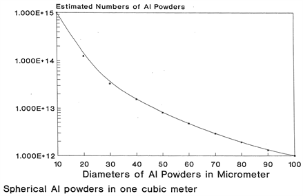
Figure 3. Relation between particle number and particle size.

Figure 4. Relation between effective surface area and particle size.
2) The density and specific heat of air at various temperatures
The density and specific heat of air at different temperature is calculated and summarized by Shih [59] [60] in Table 3 and plotted in Figure 5 and Figure 6. The specific heat of air reaches the minimum at about 273 K.
3) Viscosity of air, argon, and oxygen at various temperatures
The viscosity of air, argon, and oxygen at different temperatures is calculated and summarized in Table 4 and plotted in Figure 7 by Shih [59] [60] . The viscosity of air is less than that of oxygen and argon.
4) Calculation of heat transfer
One of the principal attractions of fluidized bed is the high rate of heat removal and addition. There are three modes of heat transfer which are of interest in gas fluidized bed.
· Gas to particle.
· Particle to particle.
· Particle to heat transfer surface.
For particles less than 1mm diameter, the overall heat transfer rate between a fluidized bed and gas entering through the distributor plater is so large that the gas attains the bed temperature within a few centimeters. For particles less than 100 μm diameter, the overall heat transfer rate between a fluidized bed and gas entering through the distributor plate is even larger that the gas attains the bed temperature within 1 centimeter. Since the high thermal conductivity of aluminum powders, the heat transfer among aluminum particles can be negligible. In fact, aluminum powders are pre-heated in argon environment and reach the temperature of the fluidization bed. Therefore, the surface-to-bed heat transfer coefficient can reach a maximum value αmax and it can maintain over a wide range of velocity above the Umf. By considering the masked surface by bubbles, the Zabrodsky correction for αmax is shown below:
(1)
For air at 200˚C
Table 3. Density and specific heat of air at various temperature.
Table 4. Viscosity of air, argon, and oxygen at different temperatures.
*: The unit of μ is (kg/m.s.) ×106 and μair = {17.4 + 0.0420 × T(˚C)}.
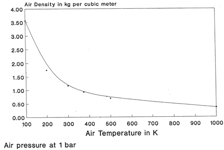
Figure 5. Air density at different temperatures.
(2)
The overall heat transfer coefficient, αo, is shown as
(3)
and
(4)
![]()
Figure 6. Specific heat of air at different temperatures.
![]()
Figure 7. Viscosity of air, argon, and oxygen at different temperatures.
Assuming the heat height of aluminum powder is about 22.0 centimeter, the total heat through the wall to the fluid of the bed can be calculated as
(5)
For a given fluidized bed from 25˚C to 200˚C as an example, the total heat is
(6)
Assuming that 1.5 pounds of aluminum powders have been pre-heated in argon environment to 200˚C, the total heat to raise air from 25˚C to 200˚C as an example at a constant flow rate is shown below:
(7)
and
(8)
The specific heat of aluminum powders at 200˚C is calculated as
(9)
and
(10)
If aluminum powders are injected to the bed in a feed rate fAl, the heat needed for aluminum powers can be calculated as
(11)
Since the volume of flow rate of air is fixed as
(12)
Therefore, one can calculate the velocity of air
(13)
and
(14)
From Equation (14), the calculated air velocity equals to the actual air velocity.
Now we should consider the required surface area of the wall to raise air from 25˚C to 200˚C. Here we have
(15)
and
(16)
Since the circumference of the reactor is
(17)
The heat length of air equals
(18)
The conclusion is that for particles with diameter less than 100 μm, air can attain the bed temperature as soon as it enters the bed. By increasing the flow rate by 100 times, Aair increases 100 times and the heat length equals 2.2 centimeters. Hair is function of Din, T, dp, V, and Jair.
5) Maximum bed height
In order to keep the fluidized bed in bubble condition without slugging, the maximum bed height (Hmax) and the inner diameter of the bed should satisfy the following relation:
(19)
For a given fluidized bed with 0.070 m inner diameter, the maximum allowable depth for 100 μm to 10 μm diameter aluminum powders, the maximum bed depth should be less than 19.7 cm and 39.3 cm, respectively (see Table 5). The maximum allowable depth of the bed decreases when the diameter of aluminum particles increases. From Equation (19), one can see that Hmax is a function of
Table 5. Relationship between diameter of aluminum powder and Hmax.
*: Equation (19) is used to estimate Hmax.
Din, ρp, and dp. The complete values of Hmax are shown below:
The relation will be used for the comparison.
(20)
and
(21)
The minimum heated length from Equation (21) is 22.0 cm and the maximum bed depth should be less or close to L to avoid slugging.
6) The Maximum bubble diameter
The maximum bubble diameter at the surface of a bed can be calculated as
(22)
Assuming the free fall velocity of the particles equals 0.1 m/sec., the maximum bubble diameter is shown below:
(23)
7) The Average particle size
The average particle size can be calculated by Equation (24)
(24)
dp is taken as 20 μm in the calculation.
8) The Height of the gently settled bed
The gently settled bed is calculated as follows:
(25)
(26)
(27)
and
(28)
The pressure of the bed is
(29)
The mass of the bed is
(30)
9) Archimedes number and minimum fluidization velocity
The basic equation to calculate Archimedes number, Ar, is as below:
(31)
and the minimum fluidization velocity is
(32)
For particles with 20 μm diameter and at 200˚C, Ar is given as
(33)
and
(34)
There are many factors which effect Archimedes number and minimum fluidization velocity. Table 6 and Table 7 show the relations among particle size, temperature, Archimedes number, and minimum fluidization velocity. Basically, at certain temperature with dv increasing, both Ar and Umf increase. For the same particle size with temperature increasing, both dv and Umf decrease. Table 6 and Table 7 show the relations of dv, Ar, and Umf at 100˚C and 200˚C, respectively [55] [56] [57] [59] [60] . Figure 8 and Figure 9 provide the Ar and Umf values for different dv, respectively [55] [56] [57] [59] [60] .
10) Thermal conductivity of air, argon, and oxygen
Table 6. Relations of particle size, archimedes number, and minimum fluidization velocity at 100˚C.
+: . *: .
Table 7. Relations of particle size, archimedes number, and minimum fluidization velocity at 200˚C.
+: . *: .
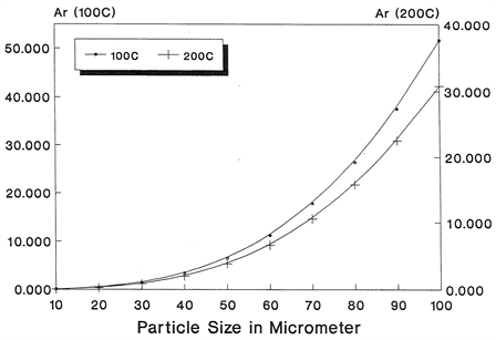
Figure 8. Relation between particle number and archimedes number.
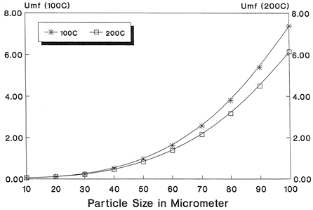
Figure 9. Relation between minimum velocity and particle size.
The thermal conductivity of air, argon, and oxygen is calculated in Table 8 and plotted in Figure 10 by Shih [59] [60] . The thermal conductivity of air and oxygen is very similar, but the conductivity of argon is much lower than the values of oxygen and air.
3. Model of Velocity and Pressure Distribution of a Gas Fluidization Bed Reactor
After the basic calculation, we can start to develop the dynamic model of velocity of pressure in the defined gas fluidization bed. The geometry of the fluidized bed is shown in Figure 11. The bed height is H in meter and the gas flow rate is Q in m3/s. There are n holes on the gas distributor, the radius of the hole is R. Assuming the particles are gently settled and when the bed is fluidized, the gas flow from the distributor forms n flow pipes through the bed with radius of the pipe equals to R. We also assume that the flow is evenly distributed among the n pipes. Therefore, the flow rate in each pipe is
(35)
From Equation (12), one has
(36)
Table 8. Thermal conductivity of gases at different Temperatures+.
+: Thermal conductivity in unit W·m−1·K−1.
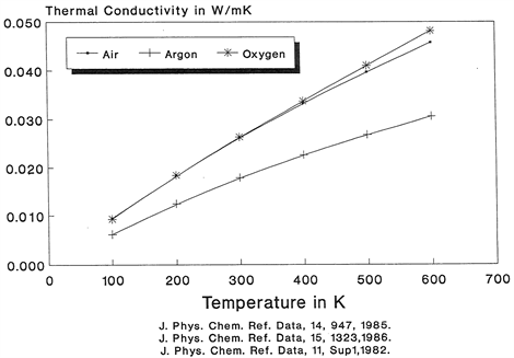
Figure 10. Thermal conductivity of air, argon, and oxygen at different temperatures.

Figure 11. The geometry of gas fluidization bed.
If n = 1000, then we have
(37)
1) Reynolds Number
Since R ≈ 10−5 m, velocity of air = 0.022 m/s and assume that the flow has a similar viscosity as air, at 200˚C, μair = 26.0 × 10⁻⁶ kg/ms, the Reynolds number is
(38)
Since Re is very small, the flow is laminar flow.
2) Governing Equations and Boundary Conditions
We chose cylindrical and Spherical coordinate system as illustrated in Figure 12. The coordinate center is at each flow pipe’s centerline on the distributor surface (Z1). Assume the flow is steady and incompressible, i.e., change of gas density is negligible, the basic equations for gas flow in the cylindrical and spherical coordinates [61] [62] are as follows:
Continuity:
(39)
R-direction momentum equation:
(40)

Figure 12. Cylindrical and spherical coordinate systems.
where
(41)
Equation (41) is the Laplace operator of Vr.
θ-direction momentum equation:
(42)
z-direction momentum equation:
(43)
Ñ2Vθ and Ñ2Vz are the Laplace operators of Vθ and Vz, respectively.
Since the radius of the pipe is very small and the bed height is much larger than the pipe’s radius, it is reasonable to say that the dominant flow velocity component is along Z direction. The rest of two components is negligible. The flow in the pipe is also axisymmetric. There two conditions can be written as
(44)
(45)
Substitute Equations (44) and (45) into continuity Equation (39) and momentum Equations (40)-(43), we have the following relations obtained
(46)
(47)
(48)
(49)
From Equation (46)
(50)
(51)
(52)
(53)
where g is the gravity.
Substitute Equations (51)-(53) into Equations (47)-(49), one obtains
(54)
(55)
(56)
From Equations (54) and (55), we know that P is only a function of Z, therefore, Equation (56) can be written as
(57)
The boundary condition at the pipe wall is
(58)
3) Solution of the Equations
Integration of Equation (57), on obtains
(59)
where C1 is an integration constant and the density ρ is assumed to be constant.
Integrate Equation (59) again, we have
(60)
where C2 is another integration constant.
At r = 0 (pipe axis), Vz is finite, therefore, using Equation (59)
(61A)
(61B)
Therefore, one has
(61C)
Substitute Equation (61C) into Equation (60), one has
(62)
In the pipe, maximum velocity occurs at r = 0
(63)
To calculate the mean velocity, we need to calculate flow rate q from the Vz distribution.
(64)
Mean velocity is shown below:
(65)
It is interesting to note that
(66)
Equation (65) can be rewritten as
(67)
Integrate Equation (67), we then have
(68)
where P1 is the pressure at the inlet of the pipe Z1.
We assume the variation of gas density inside the bed is negligible as discussed before, i.e.,
(69)
Thus, Equation (68) becomes
(70)
From Equation (70), one can see that the pressure of air depends on many factors. The factors are T, μ, ρ, Z, q, R, and Vz,mean. At a given temperature and for a fixed bed, T, μ, ρ, Z, q, and R are constants, the pressure difference is only a function of Z. The concentration of oxygen is proportional to the pressure at a Z position. Therefore, the bulk concentration of oxygen at different Z positions can be estimated using Equation (70).
4. Applications of the Mathematical Modeling and Solutions Developed
1) Calculation of air pressure in FBR.
We have the following relation as shown in Equation (70).
(70)
Assuming ;
(inlet of the FBR).
where N = m·kg/s2 and
Equation (70) becomes
(71)
Since ρ is the fluid density which equals to the density of gas phase, Vz,mean is determined by the overall flow rate in FBR and the inner diameter of the bed, Din, Z is limited by the maximum bed depth (Hmax), dynamic viscosity μ and fluid density ρ can be calculated and obtained from Program “FLOW.EXE” and FLOW1.EXE, so as to Vz,mean (Vave) and Hmax, P can be calculated using Equation (71).
Since ρ and μ are function of temperature, therefore, P is function of μ, ρ, Vz,mean, Z, T, and R and R is the radius of flow pipe. Z is also a function of particle size. We can express these relations as follows (see Equation (72)):
(72)
where Q is the overall flow rate entering the FBR, T is the temperature, and Comp is the composition of gas phase in FBR.
From Equation (72), one can see that P decreases linearly with Z increasing and the typical calculation is shown below when the following parameters are selected in the calculation:
; ; ; ; ; ; ; ; ; ; ; ; ; .
Using Equation (72), one can obtain P at different Z positions.
Case 1: When and , one obtains
(73)
The average pressure of air in the FBR bed is 0.9135 atm.
In this case, the concentration of oxygen decreases greatly in the FBR.
Case 2: When and , one obtains
(74)
The average pressure of air in the FBR bed is 0.9985 atm.
In this case, the concentration of oxygen is uniformly distributed in the FBR.
Case 3: When and , one obtains
(75)
The average pressure of air in the FBR bed is 0.9995 atm.
In this case, the concentration of oxygen is uniformly distributed in the FBR.
From the above calculation, one can get the following conclusions:
- Oxygen is uniformly distributed in a FBR with large size of particles.
- Oxygen is not uniformly distributed in a FBR with small size of particles.
- The effect of gravity to the pressure P is negligible.
2) Estimation of Diffusion Coefficient in FBR
From the theory of random walk analysis with a vacancy mechanism, one has the following relation:
(76)
where Do is specific diffusion coefficient in cm2/s; n is the nearest position of jumping; ω is the frequency to jump from a position to a specific nearest neighbor and is about 1012 to 1013 s−1; α is the jumping distance of lattice sites.
For B.C.C., and n = 8.
For F.C.C., and n = 4.
For interstitial problem, and n = 4.
Therefore, one has
(77)
(78)
(79)
Considering the correction factor fcf, Equations (77)-(79) can be written as follows:
(77F)
(78F)
(79F)
Since aluminum has a f.c.c. crystal structure and ao equals 2.86 Å, Equations (78F) holds and equals
(80)
Considering the anion vacancy mechanism, the diffusion coefficient is shown as Equation (81).
(81)
where Dv,anion is the volume diffusion coefficient of anion vacancies; ΔEtot is the total activation energy including motion and vacancies in kcal/mol; R is gas constant in 1.9872 cal/K·mol; T is the temperature in K. Do,fcc.Al is specific diffusion coefficient of f.c.c. aluminum
Generally, the activation energy is between 20 kcal/mol and 40 kcal/mol. By taking the average value of 30 kcal/mol, one obtains
(82)
(83)
(84)
(85)
Since at low temperature oxidation of aluminum powders, diffusion may also be affected by grain boundaries, the actual diffusion coefficient may be less than the values calculated in Equations (82)-(85).
3) The Effect of Oxygen Pressure to Dominant Oxide Defect
As D. D. Macdonald proposed a “dry” oxidation of aluminum [63] , aluminum oxide grows as bilayer structure. The inner layer is due to the movement of oxygen vacancies from metal/film interface and the outer layer is due to the movement of cations outward from film/environment interface. Only barrier layer is considered to contribute to passivity.
The overall reaction of the oxidation is shown as below:
(86)
The principal crystallographic defects are
1) Vacanies: , for AlO3/2.
2) Interstitials: , and .
The growth of the oxide occurs via simultaneous vacancy and electron transport. Either of them can be rate-determining step.
The reaction constant of Equation (86), , equals
(87)
Because stoichiometrically, , Equation (87) becomes
(88)
and the oxygen anion vacancy equals
(89)
Considering the cation vacancy ,
(90)
and
(91)
The effect of oxygen pressure to the dominant oxide defect can be studied by using Equations (89) and (91).
Let’s first consider the effect of oxygen pressure to oxygen anion vacancy at the worst case when aluminum powders have an average diameter as of 10 μm (see Equation (73)).
(92)
(93)
(94)
(95)
(96)
and
(97)
(98)
From the above calculation, we can conclude that oxygen pressure in FBR at current working condition has no effect to the concentration of oxygen anion vacancies. The maximum variation of oxygen anion vacancies is below 5% for aluminum spherical powders with at the 10 μm diameter as the worst case 1. The vacancy concentration increases about 5.0% at Zmax (Hmax) position (0.39 m).
For aluminum powder with 50 μm diameter or larger, oxygen pressure has no effect to both oxygen anion vacancies and cation vacancies. The maximum variation on defect concentration of 50 μm diameter aluminum powder, for example at 200˚C for both cases, is less than 0.4% (see Case 2 and Case 3 for Equations (74) and (75)).
4) Oxidation on A Planar Aluminum Surface
From the diffusion theory on a planar surface, the dependence of rate of oxidation and the thickness of the oxide film formed through diffusion can be expressed as shown in Equations (99A) and (99B).
(99A)
and
(99B)
where ξ is the thickness of the oxide, Do is the diffusion coefficient of oxygen, and r is a constant.
From Fick’s 2nd law, the diffusion of oxygen and metal is written as
(100)
(101)
where DAl is the diffusion coefficient of aluminum species, No and NAl are atomic concentrations of oxygen and aluminum species, respectively.
In order to solve the differential equations, the following boundary conditions are assumed:
(102)
(103)
(104)
(105)
where is the concentration of oxygen species at the surface and is the concentration of bulk aluminum.
By combining Equations (100)-(105), the concentrations of No and NAl are given
(106)
(107)
Let
(108)
(109)
(110)
(111)
where Jo and JAl are the flux of oxygen and aluminum species, respectively.
By combining Equations (106), (107), and (111), one obtains
(112)
From Equations (112), r may be evaluated and ξ may be calculated or compared with experimental results. For internal oxidation, the following relations may have
(113)
(114)
When or , the error and exponential functions can be simplified as
(115)
(116)
(117)
Introduction Equations (115), (116), and (117) to (112), one has
(118)
and
(119)
If is a constant and is a function of position Z, one obtains
(120)
at a fixed temperature,
(121)
where
A parabolic rate law is applied. It is associated with Wagner’s mechanism [41] [42] .
Assuming
(122)
(123)
(124)
The thickness of the oxide film after 60 minutes oxidation from Equation (121) is shown in Table 9.
Table 9. Relation between and thickness ( ) of oxide film after 60 minutes oxidation.
5) Oxidation on Spherical Aluminum Powders
General diffusion in sphere has been studied by Crank [64] , Shewmon [65] , Galus [66] , and Bitler [67] for different applications and for the FBR oxidation of aluminum powders as well as the surge arresting materials by Shih [55] [56] [57] [59] [60] [68] [69] [70] [71] [72] .
The growth rate of oxide layer can be estimated from the total amount of diffusing substance entering (oxygen lattice anions) or leaving (aluminum ions) the sphere in a gas fluidization bed considering the initial oxide thickness at time zero.
(125)
where is the amount of substance entering or leaving the sphere at time t; is the amount of substance entering or leaving the sphere at time infinite and ; is the initial amount of substance entering or leaving the sphere at time ; is a correction function due to effect of oxygen pressure to the dominant oxide defect and equals to 1.0 for spherical particle with 50 μm diameter or larger; ; is radius of aluminum powder.
is a correction function of oxygen pressure at a position Z in a gas fluidization bed and the estimation of to the dominant oxide defect can be described in two cases. Laplace transforms is used to describe the calculation of growth of oxide film and Laplace Transforms and Laplace Transforms is shown in the standard tables [73] [74] and the applications are summarized by Zhang in his book [75] . The detail deviations of Laplace Transforms of spherical aluminum powders is shown in the Appendix in this work.
Case 1: Oxygen anion vacancy is the dominant oxide defect.
The correction factor considering the oxygen vacancy concentration with oxygen pressure is shown as below:
(126)
Equation (126) is based on the linear increase of P-1/4 with Z increasing in the FBR.
For aluminum spherical powders with diameters between 10 μm and 100 μm, is very close to 1.0 and the average maximum variation of oxygen anion vacancy is +2.5%.
Case 2: Aluminum cation vacancy is the dominant oxide defect.
The correction factor considering the oxygen vacancy concentration with oxygen pressure is shown as below:
(127)
Equation (127) is based on the linear decrease of P3/4 with Z increasing in the FBR.
For aluminum spherical powders with diameters between 10 μm and 100 μm, is also very close to 1.0 and the average maximum variation of aluminum cation vacancy is −6.0%.
The typical values of and are 1.025 and 0.994 for 10 μm diamter spherical aluminum powders, respectively. Detailed calculation were generated through a computer program called “APRIL.EXE” written by Shih [59] [60] [70] . The computer program calculated the values as of Minit, Mt.cal and Dv, respectively. Equations (70) and (125) are the base of the computer software for the calculation.
For spherical aluminum powders with diameter at 50 μm or larger, both and equal 1.0. It means that the oxygen pressure is so uniform in the FBR that oxygen pressure has no effect to the concentration of the dominant oxide defects at different Z positions.
Typical calculation of oxide thickness using software “APRIL.EXE” [59] [60] [70] and the comparison between experimental thickness in the FBR and the theoretical calculation based on the dynamic model is shown the the attached tables as below.
In Table 10, the relation of Mt,exp and Mt,cal for Oxygen Anion Vacancy Mechanism is calculated using computer software “APRIL.EXE” at various temperatures when ro = 10 μm, f(ro)oxy = 1.025, and Minit = 0.00075 (25 Å) are considered.
Table 10. Relation of Mt,exp and Mt,cal for oxygen anion vacancy mechanism. Assuming , , , and cm2/s at 373 K, 473 K, 573 K, and 673 K, respectively; ; ; Minit = 0.00075 (25 Å); ; thickness of oxide = 100 Å; t = 3600 seconds. Where .
*: Mt,exp is the experimental thickness in a FBR obtained at the optimized FBR temperature based on the theoretical calculation between 473 K and 573 K.
From Table 10, the oxide layer thickness through theoretical calculation using the model developed can meet experimental oxide layer thickness in a fluidization bed between 473 K and 573 K for aluminum powders with a 10 μm diameter.
In Table 11, the relation of Mt,exp and Mt,cal for Oxygen Anion Vacancy Mechanism is calculated using computer software “APRIL.EXE” at various temperatures when ro = 60 μm, f(ro)oxy = 1.0, and Minit = 0.000125 (25 Å) are considered.
From Table 11, the oxide layer thickness through theoretical calculation using the model developed can meet experimental oxide layer thickness in a fluidization bed between 473 K and 573 K for aluminum powders with a 60 μm diameter.
In Table 12, the relation of Mt,exp and Mt,cal for Oxygen Anion Vacancy Mechanism is calculated using computer software “APRIL.EXE” at 373˚ K when ro = 10 μm, f(ro)oxy = 1.025, and Minit = 0.00075 (25 Å) are considered.
From Table 12, the oxide layer thickness through theoretical calculation using the model developed cannot meet experimental oxide layer thickness with optimized temperature when the oxidizing temperature in the calculation is only taken at 373 K for aluminum powders with a 10 mm diameter.
In Table 13, the relation of Mt,exp and Mt,cal for Oxygen Anion Vacancy
Table 11. Relation of Mt,exp and Mt,cal for oxygen anion vacancy mechanism assuming , , , and cm2/s at 373 K, 473 K, 573 K, and 673 K, respectively; ; ; Minit = 0.000125 (25 Å); ; thickness of oxide = 100 Å; t = 3600 seconds. Where .
*: Mt,exp is the experimental thickness in a FBR obtained at the optimized FBR temperature based on the theoretical calculation between 473 K and 573 K.
Table 12. Relation of Mt,exp and Mt,cal for oxygen vacancy mechanism at a fixed temperature assuming at 373 K; ro = 10 μm; ; Minit = 0.00075 (25 Å); ; thickness of oxide = 100 Å. Where .
*: Mt,exp is the experimental thickness in a FBR obtained at the optimized FBR temperature based on the theoretical calculation between 473 K and 573 K. But the target oxide layer thickness cannot be achieved in the theoretical calculation when FBR sets at 373 K.
Table 13. Relation of oxide layer thickness and oxidizing temperature at a fixed time. Assuming ro = 60 μm; time = 7200 seconds; Minit = 0.000125 (25 Å).
*: Mt,exp is the experimental thickness in a FBR obtained at the optimized FBR temperature based on the theoretical calculation between 473 K and 573 K. Mt,exp can be achieved between 520 K and 525 K.
Mechanism is calculated using computer software “APRIL.EXE” at various temperatures when ro = 60 μm, f(ro)oxy = 1.0, and Minit = 0.000125 (25 Å) are considered. The oxidizing time in the gas fluidization bed reactor is fixed as of 7200 seconds.
From Table 13, the oxide layer thickness through theoretical calculation using the model developed can definitely meet experimental oxide layer thickness where the oxidizing temperature is well-controlled in a narrow range at a fixed oxidizing time in the gas fluidization bed reactor. Between 520 K and 525 K, one can achieve a consistent oxide film thickness between experimental result and theoretical calculation.
5. Summary and Conclusions
1) The mathematical modeling considering mass, momentum, energy conservation, effects of powder size, temperature, gas velocity, and other related factors has been developed for aluminum powder oxidation in a gas fluidized bed. This is the 1st modeling for a quantitative calculation of thickness of aluminum oxide in a gas fluidization bed.
- At cross section of the pipe, the distribution of Vz is parabolic and Vz does not change along Z direction.
- Pressure is linearly decreasing along Z direction and it is proportional to the pressure of air.
2) In the mathematical model, Equations (65) and (70) as a solution can be used in the calculation of the growth rate of aluminum oxide quantitatively. Vz,mean is the mean velocity of air. The average oxidation rate of aluminum powders can be estimated from Equations (65), (70), and (125) for spherical aluminum powders and Equations (92) and (93) for planar aluminum surface.
3) The oxidation kinetics of planar and spherical aluminum powders has been discussed in great details. A uniform temperature field and a nice distribution of gas phase provide the uniform oxide growth rate of aluminum powders in the gas fluidization bed.
4) The basic theories of oxidation and growth rates have been summarized. The most possible growth rate of aluminum powders at low temperature initially is linear due to the surface boundary process or reaction is rate-determining. After initial oxidation the growth rate will follow parabolic law due to the diffusion processes in the growth of aluminum oxide. In this case, Wagner’s mechanism holds.
5) The oxidation mechanisms of aluminum powders can be determined by interstitial cations diffusion process or anion vacancies diffusion process. As an n-type semiconductor, the rate-determining process of aluminum oxide is diffusion.
6) If the oxidation is controlled by a diffusion process, the growth rate of the oxide layer can be calculated by solving partial differential equations. Mathematical models have been developed and presented in the article. The modeling of internal oxidation process has also been discussed.
7) The growth rate from the experimental results is compared with the estimation of the models developed in this article. Very good correlation between theoretical calculation and experimental results are observed.
8) The optimization of gas fluidization of the oxide of aluminum powders involve many factors which have to be considered in the theoretical analysis of mathematical modeling. The detail information can be obtained through theoretical calculation and its comparison with experimental results. A computer program written by the author has been used in the calculation. An example calculation has been shown in the technical paper at a fixed temperature, particle size, gas velocity, bulk concentration of oxygen and aluminum, Archimedes number, minimum fluidization velocity, bed depth, and effective surface area.
9) The oxidation at high temperature generates stress in the outer oxide films on aluminum particles and leads to the formation of cracks. With the increase in the intensity of crack formation, the oxidation rate increases markedly, particularly for the γ-α-Al2O3 transition. The oxidation film is not protective at high temperature oxidation. By controlling the oxidation at low temperature with the variations of oxygen concentration and relative humidity, the oxide layer is more protective and uniform.
Acknowledgements
The author would like to express thanks to Leviton Manufacturing Company for sponsoring the project through Henry Martínez and Steven Chen. The author also would like to express great thanks to Stanford Research Institute for conducting the gas fluidization bed tests to confirm the theoretical calculation and experimental results of aluminum spherical powder oxidation through Dr. Kai-Hung Lau and A. Sanjurjo. Helpful discussion with Dr. D. B. Macdonald, Dr. Richard Gottscho, and Dr. John Daugherty are greatly appreciated.
Conflicts of Interest
The author declares no conflicts of interest regarding the publication of this paper.
Cite this paper
Shih, H. (2019) Oxidation Kinetics of Aluminum Powders in a Gas Fluidized Bed Reactor in the Potential Application of Surge Arresting Materials. Materials Sciences and Applications, 10, 253-292. https://doi.org/10.4236/msa.2019.103021
References
- 1. Shih, H. (2012) A Systematic Study and Characterization of Advanced Corrosion Resistance Materials and Their Applications for Plasma Etching Processes in Semiconductor Silicon Wafer Fabrication. In: Shih, H., Ed., Corrosion Resistance, In Tech, München.
- 2. Shih, H. (2004) Materials Characterization under High Density Plasma. Keynote Presentation on American Ceramic Society, Coconut Beach, Florida.
- 3. Shih, H. (2004) A Materials Study and Characterization of Semiconductor Wafer Fabrication. Pennsylvania State University for the 2004 McFarland Award.
- 4. Shih, H. (2001) Technology Development of Materials Characterization in Wafer Fabrication Equipment. 2001 IC Equipment Supply Chain Symposium and Tainan Manufacturing Center Opening, Taiwan, 4th May 2001.
- 5. Shih, H., Han, N., Mak, S. and Yin, G. (1997) Development and Characterization of Materials for Sub-Micron Semiconductor Etch Application under High Density Plasma. 13th International Symposium on Plasma Chemistry, Beijing, 22 June 1997.
- 6. H. Shih and Ma, D. (1998) Revolutionary Chamber Materials for Metal Etch. SEMICON West Oral Presentation, Moscone Convention Center, San Francisco, California.
- 7. Shih, H. (2000) Defect Density Reduction of 0.18μm and Beyond. Presentation on SEMICON Korea, Seoul, Korea.
- 8. Shih, H. (2000) Defect Density Reduction and Productivity Enhancement for 0.18μm and Beyond. AMSEA 7th Annual Technical Seminar at Singapore, Singapore, May 2000.
- 9. Shih, H. and Daugherty, J. (2009) Systematic Study of Yttrium Oxide Coating on Anodized Aluminum Surfaces. International Thermal Spray Coating (ITSC) Conference & Exposition, Las Vegas, 4-7 May 2009.
- 10. Brace, A.W. (1992) Anodic Coating Defects—Their Causes and Cure. Technicopy Books, England.
- 11. Shih, H. and Barber, P. (2003) Materials Laboratory Development for Anodized Aluminum Study and Supplier Qualification—Part one and Part Two. Lam Research Confidential Technical Report.
- 12. Lyon, S.B., Thompson, G.E. and Johnson, J.B. (1991) Materials Evaluation Using Wet-Dry Mixed Salt-Spray Tests. In: Agarwala, V.S. and Ugiansky, G.M., Eds., New Methods for Corrosion Testing of Aluminum Alloys, ASTM STP 1134, American Society for Testing and Materials, Philadelphia, 20-31.
- 13. Shih, H. and Daugherty, J. (2009) EIS Data Explanation of Anodized Aluminum 6061-T6 after Thermal Cycling. Lam Research Confidential Technical Report, Lam Research Corporation.
- 14. Huang, Y.L., Shih, H., Huang, T.C., Daugherty, J., Wu, S., Ramanathan, S., Chang, C. and Mansfeld, F. (2008) Evaluation of the Properties of Anodized Aluminum 6061-T6 Using Electrochemical Impedance Spectroscopy (EIS). Journal of Corrosion Science, 50, 3569-3575. https://doi.org/10.1016/j.corsci.2008.09.008
- 15. Huang, Y.L., Shih, H., Daugherty, J. and Mansfeld, F. (2009) Evaluation of the Properties of Anodized Aluminum 6061 Subjected to Thermal Cycling Treatment Using Electrochemical Impedance Spectroscopy. Journal of Corrosion Science, 51, 2493-2501. https://doi.org/10.1016/j.corsci.2009.06.031
- 16. Shih, H., Outka, D. and Daugherty, J. (2006) Specification for Hard Anodized Aluminum Coatings Using Mixed Acid for Critical Chamber Components. Lam Research Specification 202-047671-001.
- 17. MIL-A-8625. Military Specification: Anodic Coatings for Aluminum and Aluminum Alloys.
- 18. Mansfeld, F., Shih, H., Greene, H. and Tsai, C.H. (1993) Analysis of EIS Data for Common Corrosion Processes. In: Scully, J.R., Silverman, D.D. and Kendig, M.W., Eds., Eds., Electrochemical Impedance: Analysis and Interpretation, ASTM STP 1188, ASTM, 23. https://doi.org/10.1520/STP18062S
- 19. Shih, H. and Mansfeld, F. (1992) Passivation in Rare Earth Metal Chlorides—A New Conversion Coating Process for Aluminum Alloys. In: Agatwala, V.S. and Ugianksy, G.M., Ed., New Methods for Corrosion Testing of Aluminum Alloys. ASTM 1134, ASTM 180-195.
- 20. Shih, H. (1994) Electrochemical Impedance Spectroscopy and Its Application for the Characterization of Anodic Layers of Aluminum Alloys on Semiconductor Manufacturing Industry. Presentation on Corrosion Asia, September 26-30, Marina Mandarin, Singapore.
- 21. Shih, H., Huang, T.C., Wu, S., Ramanathan, S. and Daugherty, J. (2006) The Development of Next Generation Anodized Aluminum—Summary of Corrosion Study during Immersion in 3.5wt% NaCl Solution for 180 Days. Lam Research Confidential Technical Report.
- 22. Shih, H. (2006) Electrochemical Impedance Spectroscopy (EIS) Technology and Applications. Lecturer for a Short Course Sponsored by the San Francisco Section of the Electrochemical Society, Crown Plaza Hotel, Milpitas, California.
- 23. Fang, Y., Outka, D. and Shih, H. (2008) TEM Analysis of Al6061-T6 Type III Anodization and the Mixed Acid Anodization. Lam Research Confidential Technical Report.
- 24. Li, S., Outka, D. and Shih, H. (2010) Cracks in Anodized Aluminum Film. Lam Research Confidential Technical Reports, August 26, 2009, September 8, 2009, November 11, 2009, February 5, 2010, September 23, 2010, November 12, 2010, and November 30.
- 25. Shih, H., Daugherty, J, Ramanathan, S., Outka, D., Fang, Y., Hayes, D., Huang, T., Holland, P., Li, S., Avoyan, A., Zhou, C., Xu, L. and Baylon, K. (2012) Challenges in Plasma Resistant Materials: Their Characterization, and Approaches in Precision Wet Cleaning. International Thermal Spray (ITSC) Conference & Exposition, 21-24 May 2012, Houston.
- 26. Shih, H., Daugherty, J, Huang, T., Outka, D., Chang, C., Fang, Y., Li, S., Xu, L., Avoyan, A., Zhou, C., Hayes, D., Wu, S., Haruff, H., Stevenson, T., Baylon, K., La Croix, C., Ronne, A., Du, Y., O’Nei, G., Casaes, R., Kim, T.W., Vahedi, V. and Gottscho, R. (2012) A Systematic Characterization of Advanced Chamber Materials for Plasma Dry Etching Processes in Semiconductor Wafer Fabrication. 1st Annual World Congress of Advanced Materials, Beijing, 6-8 June 2012, Beijing International Convention Center.
- 27. Shih, H. (2000) Mathematical Modeling and Software for Anodic Coatings of Alumimum Alloys for Semiconductor IC Industry. 1st International Conference of Young Chinese Scientists, Xiemen, 15 December 2000.
- 28. Runge, J.M. (2018) The Metallurgy of Anodizing Aluminum—Connecting Science to Practice. Springer, Berlin.
- 29. Jones, D.A. (1992) Principles and Prevention of Corrosion. Macmillan Publishing Company, New York.
- 30. Pilling, N.B. and Bedworth, R.E. (1923) Substrate Depletion Analysis and Modeling of the High Temperature Oxidation of Binary Alloys. Journal of the Institute of Metals, 29, 529.
- 31. Vermilyea, D.A. (1957) On the Mechanism of Oxidation of Metals. Acta Materialia, 5, 492-495. https://doi.org/10.1016/0001-6160(57)90087-1
- 32. Ellingham, H.J. (1944) Transactions and Communications. Journal of the Society of Chemical Industry, 63, 125-160. https://doi.org/10.1002/jctb.5000630501
- 33. Elyutin, V.P., Mitin, B.S. and Samoteykin, V.V. (1974) National Technical Information Service of US Department of Commence.
- 34. Gaskel, D.R. (1981) Introduction to Metallurgical Thermodynamics. Hemisphere Publishing Corporation, New York, 287.
- 35. Ranade, M.B. (1975) Research of Coatings or Surface Treatment of Metal Powders. IIT Research Institute, Semi-Annual Technical Report.
- 36. Kofstad, F. (1983) High-Temperature Oxidation of Metals. John Wiley & Sons, New York.
- 37. Chistyakov, Y.D. and Mendelevich, A. (1965) High-Temperature Cracking of the Oxide Film on Aluminum. Tsvetnye Metally, No. 3, 127-130.
- 38. Thiele, W. (1962) Die Oxidation von Aluminum and Aluminumlegierung Schmelzen. Aluminum, 38, 707-715.
- 39. Encyclopedia of Inorganic Materials (1977).
- 40. Hauffe, K. (1963) Reactions in Solids and on Their Surfaces. Metallurgiya, Moscow.
- 41. Zamman, G. (1920) Zeitschrift für anorganische und allgemeine Chemie, 111, 78.
- 42. Wagner, C. (1933) Zeitschrift für Physikalische Chemie, 21, 25.
- 43. Menshikov, M.V., Molchanov, S.A. and Sidorenko, A.F. (1986) Percolation Theory and Some Applications. Results of Science and Technolohy Series, VINITI, Moscow, 53-110.
- 44. Feder, J. (1988) Fractals. Plenum Press, New York.
- 45. Shklovskii, B.I. and Efros, A.L. (1984) Electric Properties of Doped Semiconductor. Springer, Berlin.
- 46. Sokolov, I.M. (1986) Dimensionalities and Other Geometric Critical Exponents in Percolation Theory. Soviet Physics Uspekhi, 29, 924-945. https://doi.org/10.1070/PU1986v029n10ABEH003526
- 47. Herega, A. (2015) Some Applications of the Percolation Theory: Brief Review and the Century Beginning. Journal of Materials Science and Engineering A, 5, 409-414.
- 48. Zenz, F.A. (1984) Fuidization Phenomena and Fluidized Bed Technology. In: Muhammad, E. and Lambert, O., Eds., Handbook of Powder Science and Technology, Van Nostrand Reinhold Company Inc., New York, 477-506.
- 49. Geldart, D. (1990) Gas Fluidization. In: Rhodes, M.J., Ed., Principle of Powder Technology, John Wiley & Sons, New York, 119-142.
- 50. Chang, T.M. and Wen, C.Y. (1966) Fluid-to-Particle Heat Transfer in Air-Fluidized Beds. Chemical Engineering Progress Symposium Series, 62, 111-117.
- 51. Wu, S.Y. and Baeyens, J. (1991) Effect of Operating Temperature on Minimum Fluidization Velocity. Powder Technology, 67, 217-220. https://doi.org/10.1016/0032-5910(91)80158-F
- 52. Formisani, B. (1991) Packing and Fluidization Properties of Binary Mixtures of Spherical Particles. Powder Technology, 66, 259-264. https://doi.org/10.1016/0032-5910(91)80039-L
- 53. Yates, J.G. and Lettieri, (2016) Fluidized-Bed Reactors: Processes and Operating Conditions. Particle Technology Series.
- 54. Feitosa, J.D. (2017) Gas Fluidization Technology. John Wiley & Sons, New York.
- 55. Shih, H. (1992) Mathematical Modeling in Smart Materials Processing in a Gas Fluidization Bed and Impedance Study. Confidential Technical Report for Leviton Manufacturing Company Inc.
- 56. Shih, H. (1993) Fluidized Bed Reactor Model & Oxidation Kinetics. Technical Report for Leviton Manufacture Company Inc.
- 57. Shih, H. (1992) Oxidation Kinetics of Aluminum Powders in a Fluidized Bed. Confidential Technical Report to Leviton Manufacturing Company.
- 58. Lau, K.H. and Sanjurjo, A. (1992) SRI Fluidized Bed Coating Work Update. Technical Report to Leviton Manufacturing Company.
- 59. Shih, H. (1992) Oxidation Mechanism of Aluminum Powders. Confidential Technical Report to Leviton Manufacturing Company.
- 60. Shih, H. (1992) Software—FLOW for the Calculation of Fluidized Bed Reactor Model and Oxidation Kinetics of Aluminum Powders in FBR. A Software Package for Leviton Manufacturing Co.
- 61. Korn, G.A. and Korn, T.M. (1968) Mathematical Handbook. McGraw-Hill Book Co., Inc., New York.
- 62. Schlichting, H. (1955) Boundary Layer Theory. Pergamon Press, New York.
- 63. Macdonald, D.D. (1992) Electric Properties of Oxidized Al Powders—Explanation of Conduction, Breakdown, and Failure Mechanism. Technical Report to Leviton Manufacturing Company.
- 64. Crank, J. (1975) The Mathematics of Diffusion. 2nd Edition, Oxford University Press, London.
- 65. Shewmom, G. (1986) Diffusion in Solid. McGraw-Hill Book Company, New York.
- 66. Galus, Z. (1976) Fundamentals of Electrochemical Analysis. John Wiley Sons Inc., New York.
- 67. Bitler, W. (1985) Kinetics of Materials—Diffusion Theory. Class Note of MASC 503, 1981-1985, The Pennsylvania State University, State College.
- 68. Shih, H. (1991) Analysis of I/V Dynamic Curves in the Study of Surge Arresting Materials. Confidential Technical Report for Leviton Manufacturing Company Inc.
- 69. Shih, H. (1991) Software Package for Analysis of I/V Dynamic Curves. Computer Software for Leviton Manufacturing Company Inc.
- 70. Shih, H. (1993) Software—APRIL for the Calculation of Fluidized Bed Reactor Model and Oxidation Kinetics of Aluminum Powders in FBR. A Software Package for Leviton Manufacturing Co.
- 71. Shih, H. (1991) Electrochemical Impedance Spectroscopy and Its Application in the Study of Surge Arresting Materials Study. Confidential Technical Report for Leviton Manufacturing Company Inc.
- 72. Shih, H. (1991) Software Package for EIS Data Analysis in the Study of Surge Arresting Materials. Computer Software for Leviton Manufacturing Company.
- 73. Roberts, G.E. and Kaufman, H. (1966) Tables of Laplace Transforms. W. B. Saunders Co., Philadelphia.
- 74. Oberhettinger, F. and Badii, L. (1973) Tables of Laplace Transforms. Springer Verlag, New York.
- 75. Zhang, W.Z. (2001) Laplace Transform—Its Principle and Application. Central Book Publisher, Taipei.
Appendix
Diffusion in sphere was studied by Crank and others. The partial diffusion equation has a standard form, but the solution depends on the initial and boundary conditions for each special case. For aluminum spherical powders in FBR, Shih provided the solution through Laplace Transformation as shown below [56] [57] .
Since the formation of aluminum oxide involves diffusion of metal interstitial cations or anion vacancies at different ranges of temperature. The differential equations can be considered in the following ways.
(A1)
(A2)
Equations (A1) and (A2) are the diffusion equations for anion vacancies and metal interstitial cations, respectively.
Considering only oxygen anion vacancies diffusion process as rate-determining step and assuming that the concentration of at metal/oxide interface keeps constant, then at steady-state which indicates
(A3)
of which the general solution is
(A4)
where A and B are constants to be determined from the boundary conditions.
If the thickness of oxide is ξ and the radius of the sphere is ro, and
(A5)
(A6)
(A7)
(A8)
(A9)
Using Laplace Transform, one has
(A10)
(A11)
where
(A12)
(A13)
Equation (A1) becomes
(A14)
or
(A15)
Let
(A16)
(A17)
and
(A18)
Therefore
(A19)
and
(A20)
at
and (A21)
at
and (A22)
We have
(A23)
and
(A24)
at , , we have
(A25)
(A26)
(A27)
with
(A28)
where
(A29)
(A30)
(A31)
Using reverse Laplace Transformation, we have
(A32)
where
(A33)
Equation (A32) can be used to estimate No(r, t) at a fixed time when ξ and ro are selected.
Nomenclature in Basic Calculation of a Gas Fluidization Bed Reactor
Symbol Explanation Unit
Aair area needed for heating air m2
Am surface area of the wall in contact with fluidized bed m2
Ar Archimedes number -
Cair specific heat of air kJ/kgK
CAl specific heat of aluminum power kJ/kgK
Cbed circumference of the reactor m
Din inner diameter of bed m
Dout outer diameter of bed m
dbd diameter of sphere having same volume as a bubble m
di arithmetic mean of adjacent sieve apertures m
dp mean sieve size of Al powder m
dv diameter of sphere particles m
fAl feed rate of aluminum powder kg/s
Q total heat rate W
Qair total heat to heat air W
QAl total heat rate to heat powders W
Qb total heat rate at fixed temperature W
Jair volume flow rate of air m3/s
Hair heat length of air m
Hmax maximum bed height m
Hset height of gently settled bed m
Mb mass of powder in bed kg
Np total particle number of powder -
Sp total surface area of powder m2
Kqz thermal conductivity of quartz W/mK
Vff free fall velocity of Al powder m/s
Tb bed temperature K
Tf fluid temperature K
αmax maximum heat wall-to-bed transfer coefficient W/m2K
αo overall heat transfer coefficient W/m2K
αf heat transfer coefficient between tube and fluid W/m2K
ρp Al particle density kg/m3
ρf density of fluid kg/m3
ρair air density kg/m3
V total superficial gas velocity m/s
Vair air flow rate kg/s
Umf minimum fluidization velocity m/s
x thickness of reactor wall (quartz) m
xi mass fraction of particles of size di -
μ viscosity kg/ms
εvoid bed voidage -
ΔP pressure drop N/m2
Nomenclature Used in Model of Velocity and Pressure Distribution
Symbol Explanation Unit
r, θ, z components of cylindrical and spherical coordinates -
Vr, Vθ, Vz velocity components corresponding to r, θ, and z -
ρ gas density kg/m3
μ gas viscosity kg/ms
ν kinematic viscosity of gas, ν = μ/ρ m2/s
P pressure N/m2
g acceleration due to gravity 9.81 m/s2
Q total flow rate entering the bed m3/s
q flow rate of the small flow pipes and and q = Q/n m3/s
R radius of flow pipe m
Re Reynolds number -
n Number of holes of gas distributors -
Mt the diffusion substance at time t kg
M¥ the diffusion substance kg
Minit the diffusion substance at time zero kg
Mt,exp the diffusion substance in fluidized bed kg
Mt,cal the diffusion substance at time t calculated kg
ro radium of aluminum spherical powders μm
f(ro) the correction function of oxygen pressure -
f(ro)oxy correction factor considering the oxygen vacancy concentration -
f(ro)cat correction factor considering aluminum cation vacancy concentration -
Dν specific volume diffusion coefficient m2/s
T time in second s
C1 integration constant -
C2 integration constant -
ξ the thickness of oxide layer m
ν ratio of oxygen atom and aluminum atom -
oxygen anion vacancy -
aluminum cation vacancy -
oxygen interstitial -
aluminum interstitial -
atomic concentration of oxygen species atoms/m3
atomic concentration of bulk aluminum atoms/m3
K reaction rate of oxide growth on planar Al -
Kc reaction constant at a fixed z position -
Do specific diffusion coefficient cm2/s
n the nearest position of jumping in random walk -
ω the frequency to jump from a position a specific nearest neighbor. 1012 to 1013 s−1
α the jumping distance of lattice sites cm
B.C.C. Body-centered cubic structure -
F.C.C. Face-centered cubic structure -
Do,bcc specific diffusion coefficient of B.C.C. cm2/s
Do,fcc specific diffusion coefficient of F.C.C. cm2/s
Do,int specific diffusion coefficient of interstitial cm2/s
Do,fcc.Al specific diffusion coefficient of aluminum of anion vacancy mechanism cm2/s
Dv,anion volume diffusion coefficient of aluminum of anion vacancy mechanism cm2/s
DEtot the total activation energy including motion and vacancies kcal/mol
R gas constant 1.9872 cal/K·mol
erf(x) error function
erfc(x) the complementary error function