Journal of Modern Physics
Vol.08 No.06(2017), Article ID:76689,30 pages
10.4236/jmp.2017.86062
Accurate Symbolic Solution of Ginzburg-Landau Equations in the Circular Cell Approximation by Variational Method: Magnetization of Ideal Type II Superconductor
O. A. Chevtchenko
HTS-powercables.nl BV, Apeldoorn, The Netherlands

Copyright © 2017 by author and Scientific Research Publishing Inc.
This work is licensed under the Creative Commons Attribution International License (CC BY 4.0).
http://creativecommons.org/licenses/by/4.0/


Received: April 30, 2017; Accepted: May 28, 2017; Published: May 31, 2017
ABSTRACT
In this paper I access the degree of approximation of known symbolic approach to solving of Ginzburg-Landau (GL) equations using variational method and a concept of vortex lattice with circular unit cells, refine it in a clear and concise way, identify and eliminate the errors. Also, I will improve its accuracy by providing for the first time precise dependencies of the variational parameters; correct and calculate magnetisation, compare it with the one calculated numerically and conclude they agree within 98.5% or better for any value of the GL parameter k and at magnetic field , which is good basis for many engineering applications. As a result, a theoretical tool is developed using known symbolic solutions of GL equations with accuracy surpassing that of any other known symbolic solution and approaching that of numerical one.
Keywords:
Ginzburg-Landau Equations, Accurate Symbolic Solution, Circular Unit Cell

1. Introduction
Much of basic superconductor behavior in magnetic field can be understood from the phenomenological model expressed by two Ginzburg-Landau (GL) equations [1] [2] . Known numerical methods produce excellent and reliable results along with “…difficulty of a numerical solution of the complex-valued GL equations” [3] [4] , the demands of calculation effort and time and being less transparent. Calculated magnetisation curves for vortex lattices with rectangular, hexagonal or circular unit cells coincide within line thickness [3] . This fact motivates solving GL equations symbolically that currently lags behind due to the complexity of the problem [5] - [10] . The lower critical field Bc1 can be accurately calculated symbolically, see Section 6.1. In strong magnetic fields the symbolic approximation [7] holds, see Section 4.2. At medium magnetic fields a symbolic approximation considering vortex lattice of circular unit cells is developed [5] [6] [8] [10] . The drawbacks of [5] [6] are dealt with in [8] [9] [10] and will not be discussed here. As stated in [8] [9] [10] , their method approximately describes magnetic properties of type II superconductors with periodic lattice over the entire range of magnetic fields and for any value of the GL parameter  with λ, ξ London penetration depth and the coherence length respectively. Moreover, the magnetic field dependence of (reversible) magnetisation can be calculated in seconds.
However, a simple check shows that magnetisation calculated with this method ( [8] [9] [10] , as published) when compared to that calculated numerically [3] , has relative differences exceeding 25%, which raises concerns about the accuracy. Clearly, the accuracy of the obtained solution of GL equations is vital: a symbolic one only has added value when its accuracy is comparable to that of the numerics. In this paper I will access the degree of approximation of the method [8] [9] [10] , refine it in a clear, concise and rational way, identify and eliminate the errors. Furthermore, I will improve accuracy of the method by providing for the first time accurate dependencies of the variational parameters; correct and calculate magnetisation, compare it with the one calculated numerically and conclude they agree for any k within 98.5% or better at magnetic field  , which is sufficient for many engineering applications.
2. Theoretical Formalism
2.1. Normalisation
In this paper I omit the time-dependent terms in the GL equations written in SI units [11] [12] and use almost the same normalisation as in [3] [11] [12] , except that I normalise all length-related quantities by the penetration depth  so that both Bc2 and
  are defined through
  and Annex provides more details. Below there are six mean (averaged over the unit cell area) magnetic field magnitudes (magnetic flux densities) in use: thermodynamic (equilibrium, applied) field Ba, magnetisation M (from the induced currents), the resulting (total) field:
 with the local field br defined by GL equations in Table 1;
the lower, the upper and thermodynamic critical magnetic fields: Bc1, Bc2 and
 respectively. Furthermore, in this paper
  is considered
independent of k or B, defined externally (through ξ and BCS theory [2] ) and at the end used as a scaling factor for all magnetic fields;  is magnetic flux quantum. Note the local magnetic flux density
 introduced (along with the four other local quantities) in Table 1 and Section 2.4. Here and below I use the dimensionless units: distance r, modulus of the magnetic vector potential
 , modulus of the super-velocity
 ,
,
![]()
Table 1. Two GL equations written in forms 1, 2 for a unit cell with axial symmetry.
magnetic induction  and
and , current density
 , magnetic flux quantum
![]() , the free energy density F and the magnitude
, the free energy density F and the magnitude ![]() of the complex GL order parameter
of the complex GL order parameter ![]() are scaled by the dimensioned units:
are scaled by the dimensioned units:![]() ,
, ![]() ,
, ![]() ,
, ![]() and
and![]() ,
, ![]() ,
, ![]() ,
, ![]() the energy density (μ0 is magnetic permeability of vacuum) and by the GL coefficients
the energy density (μ0 is magnetic permeability of vacuum) and by the GL coefficients ![]() respectively, see Table A5 for more. All dimensioned units use the International System of Units SI.
respectively, see Table A5 for more. All dimensioned units use the International System of Units SI.
2.2. Variational Method
The variational method [5] [6] [8] [9] [10] assumes for the dimensionless modulus ![]() of the complex-valued order parameter
of the complex-valued order parameter ![]() a trial function
a trial function![]() :
:
![]() (5)
(5)
where the notation ![]() is introduced; the
is introduced; the![]() ,
, ![]() are two variational parameters representing respectively the depression of the order parameter due to overlapping vortices and the effective core radius of a vortex; r, φ are the radial coordinate of cylindrical coordinate system and the phase angle respectively (a vortex line is centered on the z-axis, so that
are two variational parameters representing respectively the depression of the order parameter due to overlapping vortices and the effective core radius of a vortex; r, φ are the radial coordinate of cylindrical coordinate system and the phase angle respectively (a vortex line is centered on the z-axis, so that![]() ;
;
![]() ; x, y, z are rectangular system coordinates, etc. [8] ). Both variational parameters
; x, y, z are rectangular system coordinates, etc. [8] ). Both variational parameters ![]() and
and ![]() depend only on magnetic field
depend only on magnetic field ![]() and on the GL parameter k (Figures 1-4), so that e.g.,
and on the GL parameter k (Figures 1-4), so that e.g.,![]() . The order parameter
. The order parameter ![]() is interpreted as the local density of the Cooper pairs and its phase
is interpreted as the local density of the Cooper pairs and its phase ![]() is determined by the electric potential [12] .
is determined by the electric potential [12] .
2.3. Free Energy Density of Superconductor
Averaged over the cell area Helmholtz dimensionless free energy density F of a circular unit cell (with radius R) has two contributions [3] [8] [9] [10] :
![]() (6)
(6)
![]() (7)
(7)
![]() (8)
(8)
![]()
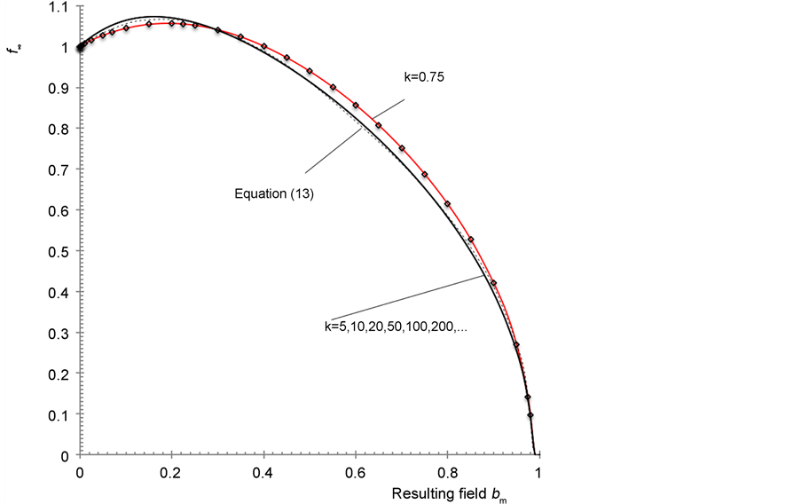
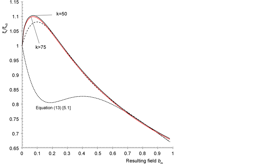
Figure 1. Calculated variational parameter ![]() vs. magnetic field bm, all dots from Annex for k ≥ 5 collapse at one curve approximated by the splines (visible here as the solid black line marked “k ≥ 5”, the dashed black line is from Equation (18) and the solid red line is the cubic spline fit at k = 0.75, indicating the range of the deviation from the curve k ≥ 5).
vs. magnetic field bm, all dots from Annex for k ≥ 5 collapse at one curve approximated by the splines (visible here as the solid black line marked “k ≥ 5”, the dashed black line is from Equation (18) and the solid red line is the cubic spline fit at k = 0.75, indicating the range of the deviation from the curve k ≥ 5).
![]()
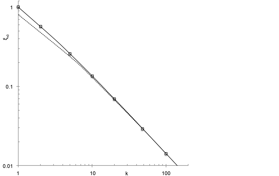
Figure 2. Calculated dependence of the variational parameter ![]() on k at
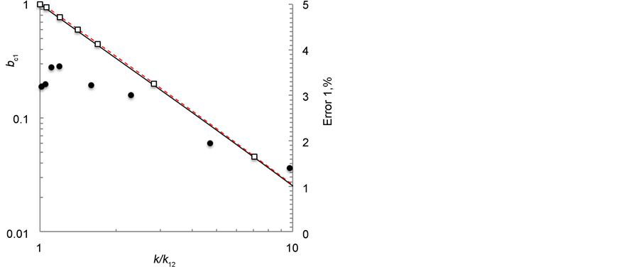
on k at![]() : the boxes represent the data from Annex (the box size corresponds to the relative error of 7%); the solid line―[ [5] , Equation (16)], the dashed line―[ [8] , Equation (15)].
: the boxes represent the data from Annex (the box size corresponds to the relative error of 7%); the solid line―[ [5] , Equation (16)], the dashed line―[ [8] , Equation (15)].
where![]() ; Fem―is related to super-current and to magnetic field; the first term of Fcore-to the local density of the Cooper pairs, and the second term:
; Fem―is related to super-current and to magnetic field; the first term of Fcore-to the local density of the Cooper pairs, and the second term:
![]() -to their interaction [2] [8] [9] [10] [13] ;
-to their interaction [2] [8] [9] [10] [13] ; ![]() is the area of the
is the area of the
circular (Wigner-Seitz) unit cell carrying one magnetic flux quantum, thus ![]()
![]() and Table A5 lists the scaling factors.
and Table A5 lists the scaling factors.
2.4. Ginzburg-Landau Equations
The GL equations are obtained by minimising the free energy of superconductor F with respect to e.g., fr and to qr (form 1, Table 1) or to fr and bkr (form 2). In the circular cell approximation both the order parameter and magnetic flux density have axial symmetry and for this case two stationary GL equations in two forms are listed in Table 1, where the five local quantities: ![]() (with
(with
![]() ),
), ![]() ,
, ![]() ,
,
![]() and
and ![]() are respectively moduli of the order parameter, of vector potential (satisfying the Coulomb gauge and having only φ-component [5] ), of local magnetic flux density vector (having only z-com- ponent), of the dimensionless super-velocity (having only φ-component), and of the vortex current density vector (having only φ-component). The two unknowns are:
are respectively moduli of the order parameter, of vector potential (satisfying the Coulomb gauge and having only φ-component [5] ), of local magnetic flux density vector (having only z-com- ponent), of the dimensionless super-velocity (having only φ-component), and of the vortex current density vector (having only φ-component). The two unknowns are: ![]() and one of the following:
and one of the following: ![]() or
or ![]() respectively for the forms 1 or 2.
respectively for the forms 1 or 2.
Complementing the Equations (1) (2) and (3) (4) Maxwell equations are:
![]() (9)
(9)
3. Solving Ginsburg-Landau Equation(s)
From Equations (4) and (5) one gets:
![]() and
and ![]() (10)
(10)
since ![]() is independent on r. Replacing the variables:
is independent on r. Replacing the variables: ![]() in Equation (10) and assuming
in Equation (10) and assuming![]() ,
, ![]() gives:
gives:
![]() , or:
, or:![]() .(11)
.(11)
Since ![]() (Section 3.4), also
(Section 3.4), also ![]() everywhere, see Equation (3). On the other hand, Equation (11) is identical to Equation (4) everywhere except at
everywhere, see Equation (3). On the other hand, Equation (11) is identical to Equation (4) everywhere except at![]() , which is the case at
, which is the case at ![]() (
(![]() ). Therefore, I conclude that at
). Therefore, I conclude that at ![]() the approach [7] must complement [8] [9] [10] as further elaborated in Section 4.2. At
the approach [7] must complement [8] [9] [10] as further elaborated in Section 4.2. At ![]() (and with
(and with ![]() independent on r) Equation (11) is the modified Bessel equation with the solution:
independent on r) Equation (11) is the modified Bessel equation with the solution:
![]() (12)
(12)
where ![]() is magnetic field strength,
is magnetic field strength, ![]() and
and ![]() are the modified Bessel’s functions respectively of the first and second kind and order 0; c1 and c2 are the integration constants set by the boundary conditions. So far the solution is the same as obtained in [8] [9] [10] . Moreover, from Equation (12) one obtains:
are the modified Bessel’s functions respectively of the first and second kind and order 0; c1 and c2 are the integration constants set by the boundary conditions. So far the solution is the same as obtained in [8] [9] [10] . Moreover, from Equation (12) one obtains:
![]() (13)
(13)
where ![]() and
and ![]() are the modified Bessel’s functions respectively of the first and second kind and order 1. Note that the derivation of the solution (Equations (10)-(13)) was skipped in [8] [9] [10] and as a result, the important restriction
are the modified Bessel’s functions respectively of the first and second kind and order 1. Note that the derivation of the solution (Equations (10)-(13)) was skipped in [8] [9] [10] and as a result, the important restriction ![]() of the solution was hidden so far.
of the solution was hidden so far.
3.1. Boundary Conditions
The boundary conditions can be found e.g., in [3] [5] [6] [8] - [13] . From there a variety follows of the definitions for c1 and c2, such as based upon [8] [9] [10] [13] : 1) quantisation of magnetic flux through the unit cell: ![]() and 2) zero current at its interface
and 2) zero current at its interface![]() :
:
![]() (14)
(14)
![]() (15)
(15)
In order to stay focused and limit the size of the paper, below I simply accept Equations (14), (15) and will study namely this case in more detail. With the constants c1 and c2 defined, the solution allows calculating the local quantities as well as the mean quantities: equilibrium magnetic field, magnetisation, etc. In this paper I focus on magnetisation.
3.2. Variational Method
In the variational method Equation (5) in fact replaces the unknown ![]() (which is otherwise obtained by solving the GL equations) and thus eliminates solving the first GL equation; instead one focuses on solving e.g., for
(which is otherwise obtained by solving the GL equations) and thus eliminates solving the first GL equation; instead one focuses on solving e.g., for ![]() (second GL equation) and for
(second GL equation) and for![]() ,
,![]() . While drawbacks of the approach [5] [6] are treated in [8] [9] [10] , I find that all three publications [8] [9] [10] are not easy to read as in turn they have crucial errors preventing the reader from wider use of this otherwise excellent method. For instance, in [8] [9] and [10] at least Equations (11), (13), (15); (22), (24), (28) and (2.18), (2.20) respectively have errors that can be decisive for the result. These errors are eliminated here and correct equations are presented thus facilitating broader use of the method. The analytical expressions for the energy density associated with the change in the order parameter near centers of vortices (Equations (15) [6] and (12) [8] respectively) though they look slightly different, are identical. On the other hand, Equation (20) of [9] is a substantial improvement of corresponding Equation (14) of [6] as it is explained in [8] [9] [10] (note that the corresponding Equation (11) [8] contains a typing error, the correct equations are: (2.16) in [10] , (20) in [9] and Equation (16) here).
. While drawbacks of the approach [5] [6] are treated in [8] [9] [10] , I find that all three publications [8] [9] [10] are not easy to read as in turn they have crucial errors preventing the reader from wider use of this otherwise excellent method. For instance, in [8] [9] and [10] at least Equations (11), (13), (15); (22), (24), (28) and (2.18), (2.20) respectively have errors that can be decisive for the result. These errors are eliminated here and correct equations are presented thus facilitating broader use of the method. The analytical expressions for the energy density associated with the change in the order parameter near centers of vortices (Equations (15) [6] and (12) [8] respectively) though they look slightly different, are identical. On the other hand, Equation (20) of [9] is a substantial improvement of corresponding Equation (14) of [6] as it is explained in [8] [9] [10] (note that the corresponding Equation (11) [8] contains a typing error, the correct equations are: (2.16) in [10] , (20) in [9] and Equation (16) here).
From Equation (12) at![]() ,
, ![]() follows and since
follows and since![]() , one gets (from Equations (6)-(8), (14) (15) here) [5] [6] [8] [9] [10] :
, one gets (from Equations (6)-(8), (14) (15) here) [5] [6] [8] [9] [10] :
![]() (16)
(16)
![]() (17)
(17)
with ![]() and
and![]() .
.
Minimising the free energy density F of superconductor, Equations (6)-(8), (16) (17), with respect to the variational parameters ![]() and
and ![]() (at fixed k and
(at fixed k and![]() ) allows establishing dependencies of
) allows establishing dependencies of ![]() and
and ![]() on k and
on k and ![]() in a self-sufficient way [5] [6] [8] [9] [10] , see detailed in Figures 1-4 and Annex. Once these are established, the order parameter is defined (Equation (5)) and the dependence of magnetisation on k and
in a self-sufficient way [5] [6] [8] [9] [10] , see detailed in Figures 1-4 and Annex. Once these are established, the order parameter is defined (Equation (5)) and the dependence of magnetisation on k and ![]() follows, see Equations (20)-(23) (24). In [5] [6] [8] [9] [10] , the accurate dependencies of
follows, see Equations (20)-(23) (24). In [5] [6] [8] [9] [10] , the accurate dependencies of ![]() and
and ![]() on k and
on k and ![]() are missing, instead inaccurate interpolation fits are published in both cases as explained below and clear from Figures 1-4. This prevents accurate calculation of magnetisation in particular. In this paper the minimising of F is done numerically (using Solver in Excel), results are presented in a clear, traceable form and in more detail as compared to [5] [6] [8] [9] [10] and they yield the following.
are missing, instead inaccurate interpolation fits are published in both cases as explained below and clear from Figures 1-4. This prevents accurate calculation of magnetisation in particular. In this paper the minimising of F is done numerically (using Solver in Excel), results are presented in a clear, traceable form and in more detail as compared to [5] [6] [8] [9] [10] and they yield the following.
3.3. Variational Parameter f∞
At any ![]() all obtained data points of the dependence
all obtained data points of the dependence ![]() collapse at one curve fitted here by a cubic spline, see Figure 1 and Table A1. For this reason no data for the individual splines is given here for this range. This simplification causes an estimated error of 0.5% as explained in Section 5 and the error can be reduced by using more accurate data from the minimising of F. Furthermore, the obtained data are in reasonable agreement with that from [ [8] , Equation (14)] (numbered as Equation (18) here), except at lower
collapse at one curve fitted here by a cubic spline, see Figure 1 and Table A1. For this reason no data for the individual splines is given here for this range. This simplification causes an estimated error of 0.5% as explained in Section 5 and the error can be reduced by using more accurate data from the minimising of F. Furthermore, the obtained data are in reasonable agreement with that from [ [8] , Equation (14)] (numbered as Equation (18) here), except at lower
(![]() ) and at higher (
) and at higher (![]() ) fields, see Figure 1:
) fields, see Figure 1:
![]() (18)
(18)
At ![]() the obtained dots deviate from this curve and the error when using Equation (18) can reach 5% as Figure 1 exemplifies. Therefore in this range instead of using Figure 1 or Equation (18), I recommend using Figure 1 or more accurately the data from Annex e.g., by constructing the individual splines. Importance of this correction becomes clear in Section 5. For the above reasons I am convinced that Equation (18) does not approximate the dependence of
the obtained dots deviate from this curve and the error when using Equation (18) can reach 5% as Figure 1 exemplifies. Therefore in this range instead of using Figure 1 or Equation (18), I recommend using Figure 1 or more accurately the data from Annex e.g., by constructing the individual splines. Importance of this correction becomes clear in Section 5. For the above reasons I am convinced that Equation (18) does not approximate the dependence of ![]() with “an accuracy of about 0.5% for arbitrary k and b” as stated in [8] [9] [10] . In addition, I find unsatisfactory the agreement of the obtained data with the Equation (24) of [6] :
with “an accuracy of about 0.5% for arbitrary k and b” as stated in [8] [9] [10] . In addition, I find unsatisfactory the agreement of the obtained data with the Equation (24) of [6] :
![]() .
.
3.4. Variational Parameter ξv
Minimisation of F with respect to ![]() at
at ![]() shows that Equation (15) of [8] is less accurate than the original Equation (16) of [5] , especially at k < 10 (and that the error exceeds 1% up to k = 50), see Figure 2. Therefore, the correct equation to calculate the dependence
shows that Equation (15) of [8] is less accurate than the original Equation (16) of [5] , especially at k < 10 (and that the error exceeds 1% up to k = 50), see Figure 2. Therefore, the correct equation to calculate the dependence ![]() for
for ![]() at any k in an ideal type II superconductor is [5] :
at any k in an ideal type II superconductor is [5] :
![]() (19)
(19)
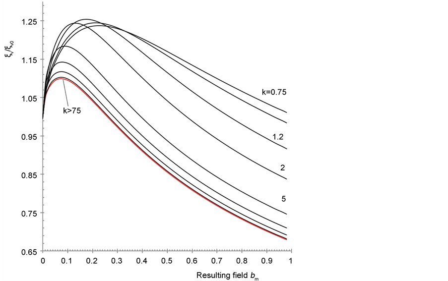
The obtained (by minimizing F) dependence ![]() is similar and different from those described in [3] [5] . On one hand at
is similar and different from those described in [3] [5] . On one hand at ![]() all data points collapse practically at one curve, see Figure 3 and Table A2 in Annex. For this reason only one cubic spline fit (namely, k = 100) is shown, the error of this simplification is below 0.5%.
all data points collapse practically at one curve, see Figure 3 and Table A2 in Annex. For this reason only one cubic spline fit (namely, k = 100) is shown, the error of this simplification is below 0.5%.
The agreement of the obtained data with [ [8] , Equation (13)] is unsatisfactory, see Figure 3 and therefore I recommend calculating ![]() for
for ![]() and any value of magnetic field
and any value of magnetic field ![]() from the spline fit, Figure 3 and Table A2 in Annex.
from the spline fit, Figure 3 and Table A2 in Annex.
On the other hand at ![]() the obtained dependence
the obtained dependence ![]() is rather different from those described in [5] [6] [8] [9] [10] and from the single curve
is rather different from those described in [5] [6] [8] [9] [10] and from the single curve ![]() in Figure 3. For instance, the relative difference for k = 50 and 0.75 reaches 50% as Figure 4 shows.
in Figure 3. For instance, the relative difference for k = 50 and 0.75 reaches 50% as Figure 4 shows.
Based on this study, I conclude that none of the Equations (13)-(15) in [8] (repeated as (22)-(24) in [9] and as (2.18)-(2.20) in [10] ) is accurate for arbitrary values of ![]() and over the entire range of magnetic fields
and over the entire range of magnetic fields![]() . Instead I recommend using more accurate data from this paper, see Annex. The most accurate results are obtained through minimising the free energy density F of superconductor with respect to the variational parameters
. Instead I recommend using more accurate data from this paper, see Annex. The most accurate results are obtained through minimising the free energy density F of superconductor with respect to the variational parameters ![]() and
and ![]() as described in this paper. This step is a must when aiming at the agreement better than 1% between magnetisation calculated symbolically and numerically, see Section 5.
as described in this paper. This step is a must when aiming at the agreement better than 1% between magnetisation calculated symbolically and numerically, see Section 5.
4. Magnetisation (Derived Symbolically)
4.1. Variational Approach
The applied (thermodynamic, equilibrium) magnetic field ![]()
from Equations (14)-(17) according to [5] [6] [8] [9] [10] is:
![]() (20)
(20)
with [8] :
![]() (21)
(21)
![]() (22)
(22)
![]() (23)
(23)
![]() (24)
(24)
and![]() . Since Equations (21)-(24) define the applied field
. Since Equations (21)-(24) define the applied field![]() , the magnetisation is:
, the magnetisation is:
![]() or:
or: ![]()
![]() (25)
(25)
Finally, after re-normalisation of Equation (25), one obtains:
![]() with
with ![]() (26)
(26)
Namely the magnetization ![]() calculated from Equation (25) after correcting the error (see Section 4.2) becomes the magnetization
calculated from Equation (25) after correcting the error (see Section 4.2) becomes the magnetization ![]() compared in Section 5 to those calculated numerically and with other symbolic methods.
compared in Section 5 to those calculated numerically and with other symbolic methods.
4.2. The Error and the Correction
The error (present in Equations (10)-(26) at![]() , see. Equations (10)-(11)) is evident from the Abrikosov solution of the linearized GL equations [7] stating:
, see. Equations (10)-(11)) is evident from the Abrikosov solution of the linearized GL equations [7] stating:
![]() (27)
(27)
for any k and ![]() with
with ![]() equal to 1.1803 (1.1596) for the vortex lattice with square (hexagonal) unit cells [4] and to 1.1576 for the lattice with circular
equal to 1.1803 (1.1596) for the vortex lattice with square (hexagonal) unit cells [4] and to 1.1576 for the lattice with circular
cells [9] ;![]() ,
,![]() . As the examples in Section 5 will illustrate, at
. As the examples in Section 5 will illustrate, at
![]() the line 5 ( [8] [9] [10] representing the magnetisation calculated from Equations (25) (26) without corrections) crosses the line 4 representing the m4 and moreover it crosses the horizontal axis at 0.985 (instead of at 1 as Equation (27) implies). The error in
the line 5 ( [8] [9] [10] representing the magnetisation calculated from Equations (25) (26) without corrections) crosses the line 4 representing the m4 and moreover it crosses the horizontal axis at 0.985 (instead of at 1 as Equation (27) implies). The error in ![]() is visible at least at
is visible at least at![]() .
.
In this paper the error is eliminated in the following way. The Equations (21)-(26) are only valid at![]() , see Equation (11). Otherwise, Equation (27) is the correct symbolic solution of GL equation(s) providing the missing additional conditions to Equations (21)-(26) and simply stating that in the plane
, see Equation (11). Otherwise, Equation (27) is the correct symbolic solution of GL equation(s) providing the missing additional conditions to Equations (21)-(26) and simply stating that in the plane ![]() the point mc2 on the true magnetisation curve
the point mc2 on the true magnetisation curve ![]() has the following coordinates:
has the following coordinates:![]() , in other words:
, in other words: ![]() and at
and at ![]()
![]() (28)
(28)
the 1st derivative through this point of the true magnetisation curve should be constant set by Equation (28) and that only depends on k and on the Abrikosov parameter ![]() [7] . Moreover, using Equation (30) and
[7] . Moreover, using Equation (30) and ![]() (that follows from the minimising the free energy in Equations (16) (17)), we can now define more accurately the vague condition “
(that follows from the minimising the free energy in Equations (16) (17)), we can now define more accurately the vague condition “![]() ” (or “
” (or “![]() ” [3] ) as:
” [3] ) as:
![]() with
with ![]() being defined by the condition:
being defined by the condition:![]() . (29)
. (29)
From [ [7] , Equation (19)] it is clear that at ![]() the free energy density (see Equations (6)-(8)) is (at minimum when
the free energy density (see Equations (6)-(8)) is (at minimum when ![]() is as close to 1 as possible):
is as close to 1 as possible):
![]() (30)
(30)
From Equations (30) and (16) (17) it is easy to check that for![]() ,
, ![]() at
at ![]() always
always![]() , which means that in this range Equation (27) is more accurate than Equation (26). On the other hand, at
, which means that in this range Equation (27) is more accurate than Equation (26). On the other hand, at
![]() Equation (26) is more accurate than Equation (27), since here
Equation (26) is more accurate than Equation (27), since here ![]() (with
(with ![]() obtained by minimising F, see Equations (16) (17)). More generally, Equation (27) must be used at
obtained by minimising F, see Equations (16) (17)). More generally, Equation (27) must be used at ![]() instead of Equation (26).
instead of Equation (26).
A smooth transition from Equation (26) to Equation (27) can be achieved in several ways. In this paper I use the following approach. So far calculated from Equation (26) magnetisation![]() . Thus Equation (26) produces the erroneous value of the upper critical field
. Thus Equation (26) produces the erroneous value of the upper critical field ![]() (see Section 6.2) due to ignoring the restriction
(see Section 6.2) due to ignoring the restriction![]() , see the condition by Equations (10) and (11). Replacing
, see the condition by Equations (10) and (11). Replacing ![]() by
by ![]() (Equation (33)) when plotting
(Equation (33)) when plotting ![]() satisfies the condition set by Equation (27) at
satisfies the condition set by Equation (27) at![]() :
:![]() . This step shifts the entire magnetisation curve (Equation (26)) parallel to itself and slightly to the right as exemplified in Section 5. Moreover, at
. This step shifts the entire magnetisation curve (Equation (26)) parallel to itself and slightly to the right as exemplified in Section 5. Moreover, at ![]() calculated from Equation (26) magnetisation should have the same first derivative as set by Equation (28). This is obviously not the case as one can see in Section 5 (not only magnetisation curve calculated from [8] [9] [10] crosses the horizontal axis at
calculated from Equation (26) magnetisation should have the same first derivative as set by Equation (28). This is obviously not the case as one can see in Section 5 (not only magnetisation curve calculated from [8] [9] [10] crosses the horizontal axis at![]() , but it has the slope different from that set by Equation (27)).
, but it has the slope different from that set by Equation (27)).
In this paper a compliance with this condition (Equation (28)) is achieved by introducing the correction:![]() , where
, where ![]() comes from Equation (26). This correction slightly rotates the entire magnetisation curve around the point
comes from Equation (26). This correction slightly rotates the entire magnetisation curve around the point![]() , so that the derivative of the magnetisation m1 becomes equal to that set by Equation (28) and the transition from m1 to m4 is smooth since the higher derivatives are preserved. Furthermore, used for the comparison (in Section 5) magnetisation m2 from [ [3] , Figure 7] is calculated numerically for the triangular vortex lattice, while the obtained here results are for the vortex lattice of circular cells, therefore accounting the respective ratio of the Abrikosov parameters (Equation (27)), more accurately:
, so that the derivative of the magnetisation m1 becomes equal to that set by Equation (28) and the transition from m1 to m4 is smooth since the higher derivatives are preserved. Furthermore, used for the comparison (in Section 5) magnetisation m2 from [ [3] , Figure 7] is calculated numerically for the triangular vortex lattice, while the obtained here results are for the vortex lattice of circular cells, therefore accounting the respective ratio of the Abrikosov parameters (Equation (27)), more accurately: ![]() in this case. Clearly, more sophisticated methods of achieving the same result can be used (all required math for combining the solutions is present e.g., in [13] ), but they are beyond the scope of this paper.
in this case. Clearly, more sophisticated methods of achieving the same result can be used (all required math for combining the solutions is present e.g., in [13] ), but they are beyond the scope of this paper.
In conclusion, the correction makes the obtained solution compliant with [7] [13] (the same point mc2 and the same direction of the magnetisation curve at this point). It should be noted that this correction of the magnetisation uses the symbolic form of the theoretical result [7] at ![]() and therefore the solution obtained here remains self-sufficient (even though it now uses two solutions of GL equations: [8] [9] [10] and [7] ). So far I did not use any numerical results (the fact that calculated numerically magnetisation m2 also agree with the conditions of Equations (27), (28) only means that these conditions are just). Corrected this way magnetisation m1 is in excellent agreement with the conditions of Equations (27), (28) and is further compared to that calculated numerically (and with other symbolic methods) in Figures 5-8.
and therefore the solution obtained here remains self-sufficient (even though it now uses two solutions of GL equations: [8] [9] [10] and [7] ). So far I did not use any numerical results (the fact that calculated numerically magnetisation m2 also agree with the conditions of Equations (27), (28) only means that these conditions are just). Corrected this way magnetisation m1 is in excellent agreement with the conditions of Equations (27), (28) and is further compared to that calculated numerically (and with other symbolic methods) in Figures 5-8.
5. Comparison and Discussion
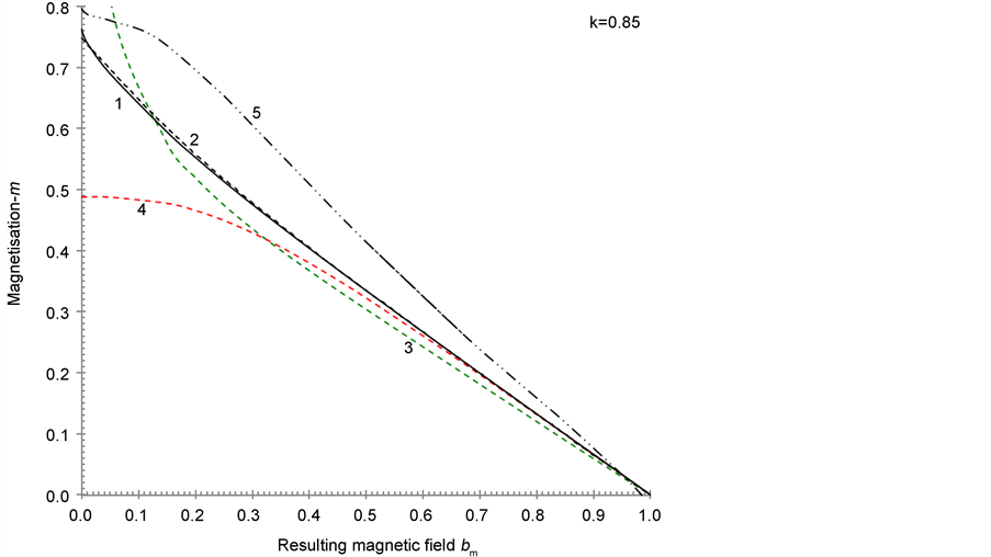
In Figures 5-8 the magnetisation m1 is compared to that calculated numerically [3] and to those calculated symbolically [7] [8] [9] [10] through the entire range of magnetic fields ![]() and representative range of the GL parameter
and representative range of the GL parameter
![]() (same range as in [3] ). In each figure the magnetisation changes between 0 and
(same range as in [3] ). In each figure the magnetisation changes between 0 and ![]() (further defined in Section 6.1). Moreover, in this range of k the
(further defined in Section 6.1). Moreover, in this range of k the ![]() changes by more than 4 orders in magnitude: between 1 and
changes by more than 4 orders in magnitude: between 1 and![]() . An overview can be found elsewhere [3] [4] of the general features of reversible magnetisation, of its dependence on k and on magnetic field, etc. as follows from numerical solving of GL equations and these are not discussed here. Instead, I focus on the validation of the obtained analytical solution (Equations (20)-(26) complemented by Equations (27)-(30) and with the data in Figures 1-4 and Annex). This is achieved by comparing magnetization m1 to magnetisation calculated using other methods. Namely, in Figures 5-8 I compare m1 to m2 - m5 being respectively magnetisation calculated from: this work (m1); [3] [4] , numerically for hexagonal unit cells (m2); [ [3] , Equation (19)] from the interpolation fit for m2 with limited validity (m3); [7] , Equation (27) here (m4) and [8] [9] [10] as published (m5).
. An overview can be found elsewhere [3] [4] of the general features of reversible magnetisation, of its dependence on k and on magnetic field, etc. as follows from numerical solving of GL equations and these are not discussed here. Instead, I focus on the validation of the obtained analytical solution (Equations (20)-(26) complemented by Equations (27)-(30) and with the data in Figures 1-4 and Annex). This is achieved by comparing magnetization m1 to magnetisation calculated using other methods. Namely, in Figures 5-8 I compare m1 to m2 - m5 being respectively magnetisation calculated from: this work (m1); [3] [4] , numerically for hexagonal unit cells (m2); [ [3] , Equation (19)] from the interpolation fit for m2 with limited validity (m3); [7] , Equation (27) here (m4) and [8] [9] [10] as published (m5).
As clear from Figures 5-8, for any value of the GL parameter ![]() and over the entire range of magnetic fields
and over the entire range of magnetic fields ![]() excellent agreement be-
excellent agreement be-
tween m1 and m2 is achieved: the relative difference ![]() is below 1.5%
is below 1.5%
everywhere (except in the narrow range: ![]() where it is below 4%, see further elaborated in Section 6.1).
where it is below 4%, see further elaborated in Section 6.1).
5.1. Ginzburg-Landau Parameter ![]()
Representative for the range of ![]() (with
(with![]() , see [ [3] , Figure 1]) set of the magnetisation curves at k = 0.85 is shown in Figure 5(a).
, see [ [3] , Figure 1]) set of the magnetisation curves at k = 0.85 is shown in Figure 5(a).
The relative difference ![]() is below 1.5% in the entire range
is below 1.5% in the entire range
![]() (except in the range:
(except in the range: ![]() where it is below 4%, see further elaborated in Section 6.1). As expected [3] , the interpolation fit (m3) to-
where it is below 4%, see further elaborated in Section 6.1). As expected [3] , the interpolation fit (m3) to-
tally fails to describe the data (m2) quantitatively, since k < 3 and thus ![]()
is too high. The data represented by magnetisation m1 (and m2) are in good
agreement with these represented by m4 at ![]() (so that both
(so that both ![]() and
and ![]() e.g., at
e.g., at ![]() are below 0.7%, even though
are below 0.7%, even though ![]() as k < 1 in
as k < 1 in
![]() (a)
(a)![]() (b)
(b)
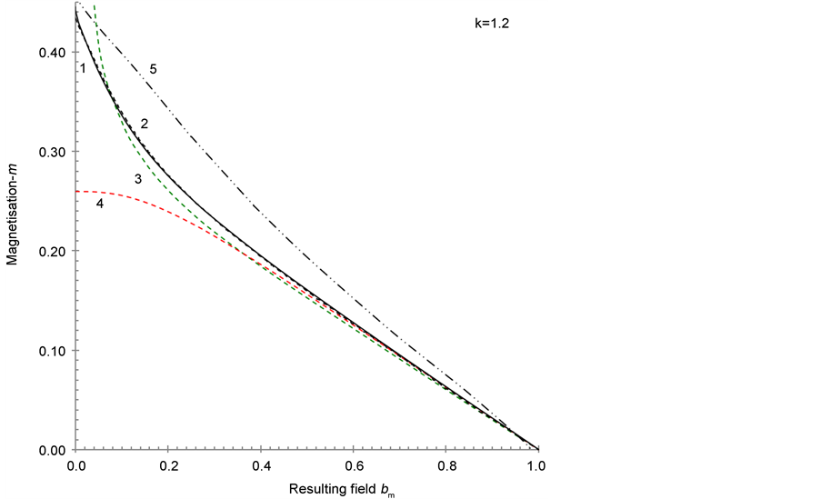
Figure 5. (a). Calculated for k = 0.85 magnetisation m as function of the resulting field![]() : 1―as proposed here (m1); 2, 3―from the numerical solution, the dashed black line (m2) restored from [ [3] , Figure 7] and the dashed green line (m3) from the fit―[ [3] , Equation (19)]; 4―from Equation (27) (m4); 5―from [8] [9] [10] (dashed double dotted line, m5). (b). Calculated for k = 1.2 magnetisation m as function of the resulting field
: 1―as proposed here (m1); 2, 3―from the numerical solution, the dashed black line (m2) restored from [ [3] , Figure 7] and the dashed green line (m3) from the fit―[ [3] , Equation (19)]; 4―from Equation (27) (m4); 5―from [8] [9] [10] (dashed double dotted line, m5). (b). Calculated for k = 1.2 magnetisation m as function of the resulting field![]() : 1―as proposed here (m1); 2, 3―from the numerical solution, the dashed black line (m2) restored from [ [3] , Figure 7] and the dashed green line (m3) from the fit―[ [3] , Equation (27)]; 4―from Equation (27) (m4); 5―from [8] [9] [10] (dashed double dotted line, m5). The line numbering is the same as in Figure 5(a).
: 1―as proposed here (m1); 2, 3―from the numerical solution, the dashed black line (m2) restored from [ [3] , Figure 7] and the dashed green line (m3) from the fit―[ [3] , Equation (27)]; 4―from Equation (27) (m4); 5―from [8] [9] [10] (dashed double dotted line, m5). The line numbering is the same as in Figure 5(a).
![]() (a)
(a)![]() (b)
(b)
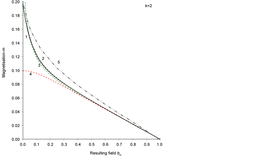
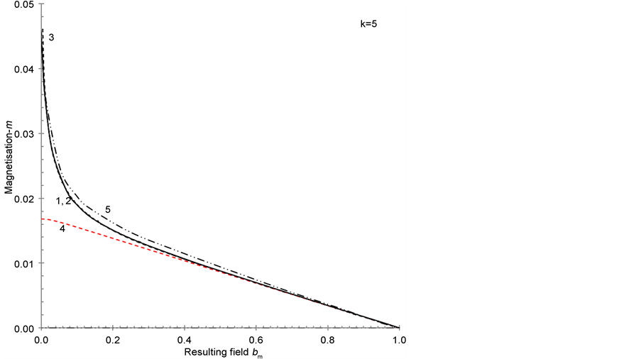
Figure 6. (a) Calculated for k = 2 magnetisation m as function of the field![]() : 1―as proposed here (m1); 2, 3―from the numerical solution, the dashed black line (m2) restored from [ [3] , Figure 7] and the dashed green line (m3) from the fit―[ [3] , Equation (19)]; 4―from Equation (27) (m4); 5―from [8] [9] [10] (dashed double dotted line, m5). The line numbering is the same as in Figure 5(a). (b). Calculated for k = 5 magnetisation m as function of the field
: 1―as proposed here (m1); 2, 3―from the numerical solution, the dashed black line (m2) restored from [ [3] , Figure 7] and the dashed green line (m3) from the fit―[ [3] , Equation (19)]; 4―from Equation (27) (m4); 5―from [8] [9] [10] (dashed double dotted line, m5). The line numbering is the same as in Figure 5(a). (b). Calculated for k = 5 magnetisation m as function of the field![]() : 1―as proposed here (m1); 2, 3―from the numerical solution, the dashed black line (m2) restored from [ [3] , Figure 7] and the dashed green line (m3) from the fit―[ [3] , Equation (19)]; 4―from Equation (27) (m4); 5―from [8] [9] [10] (dashed double dotted line, m5). The line numbering is the same as in Figure 5(a).
: 1―as proposed here (m1); 2, 3―from the numerical solution, the dashed black line (m2) restored from [ [3] , Figure 7] and the dashed green line (m3) from the fit―[ [3] , Equation (19)]; 4―from Equation (27) (m4); 5―from [8] [9] [10] (dashed double dotted line, m5). The line numbering is the same as in Figure 5(a).
![]() (a)
(a)![]() (b)
(b)
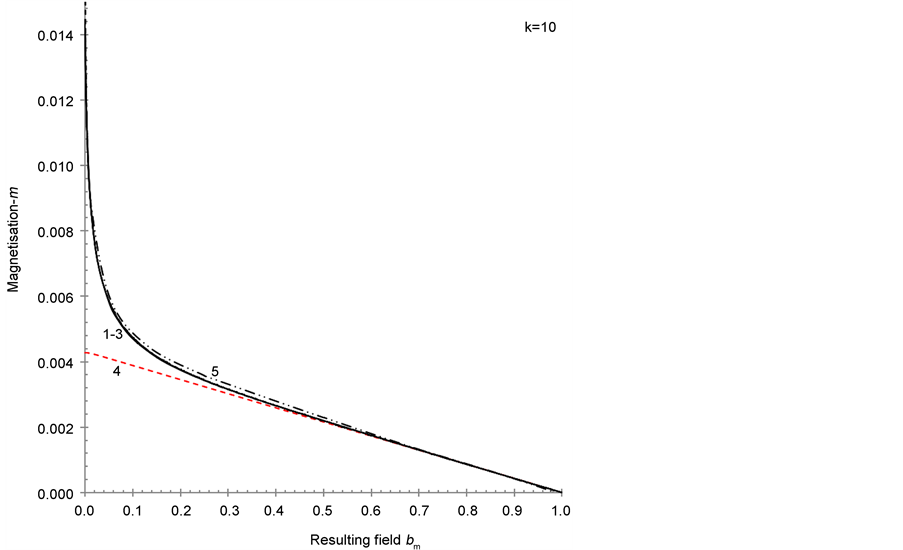
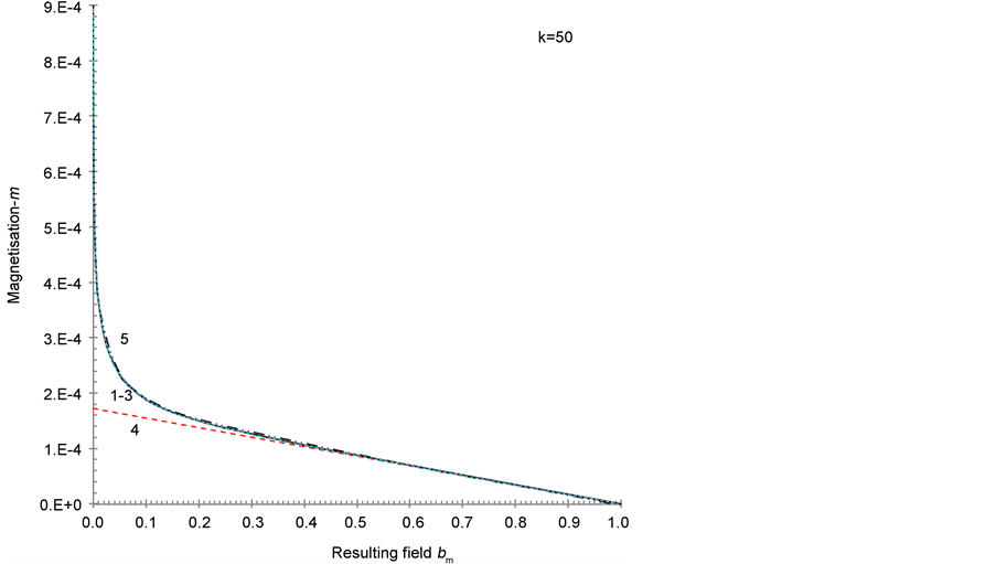
Figure 7. (a) Calculated for k = 10 magnetisation m as function of the field![]() : 1―as proposed here (m1); 2, 3―from the numerical solution, the dashed black line (m2) restored from [ [3] , Figure 7] and the dashed green line (m3) from the fit―[ [3] , Equation (19)]; 4―from Equation (27) (m4); 5―from [8] [9] [10] (dashed double dotted line, m5). The line numbering is the same as in Figure 5(a). (b) Calculated for k = 50 magnetisation m as function of the field
: 1―as proposed here (m1); 2, 3―from the numerical solution, the dashed black line (m2) restored from [ [3] , Figure 7] and the dashed green line (m3) from the fit―[ [3] , Equation (19)]; 4―from Equation (27) (m4); 5―from [8] [9] [10] (dashed double dotted line, m5). The line numbering is the same as in Figure 5(a). (b) Calculated for k = 50 magnetisation m as function of the field![]() : 1―as proposed here (m1); 2, 3―from the numerical solution, the dashed black line (m2) restored from [ [3] , Figure 7] and the dashed green line (m3) from the fit―[ [3] , Equation (19)]; 4―from Equation (27) (m4); 5―from [8] [9] [10] (dashed double dotted line, m5). The line numbering is the same as in Figure 5(a).
: 1―as proposed here (m1); 2, 3―from the numerical solution, the dashed black line (m2) restored from [ [3] , Figure 7] and the dashed green line (m3) from the fit―[ [3] , Equation (19)]; 4―from Equation (27) (m4); 5―from [8] [9] [10] (dashed double dotted line, m5). The line numbering is the same as in Figure 5(a).
![]() (a)
(a)![]() (b)
(b)![]() (c)
(c)
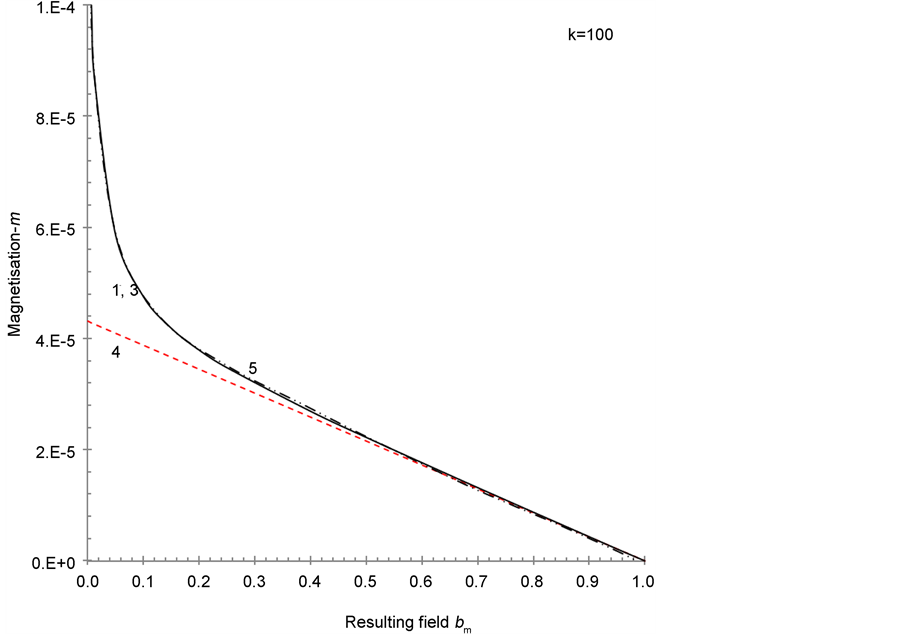
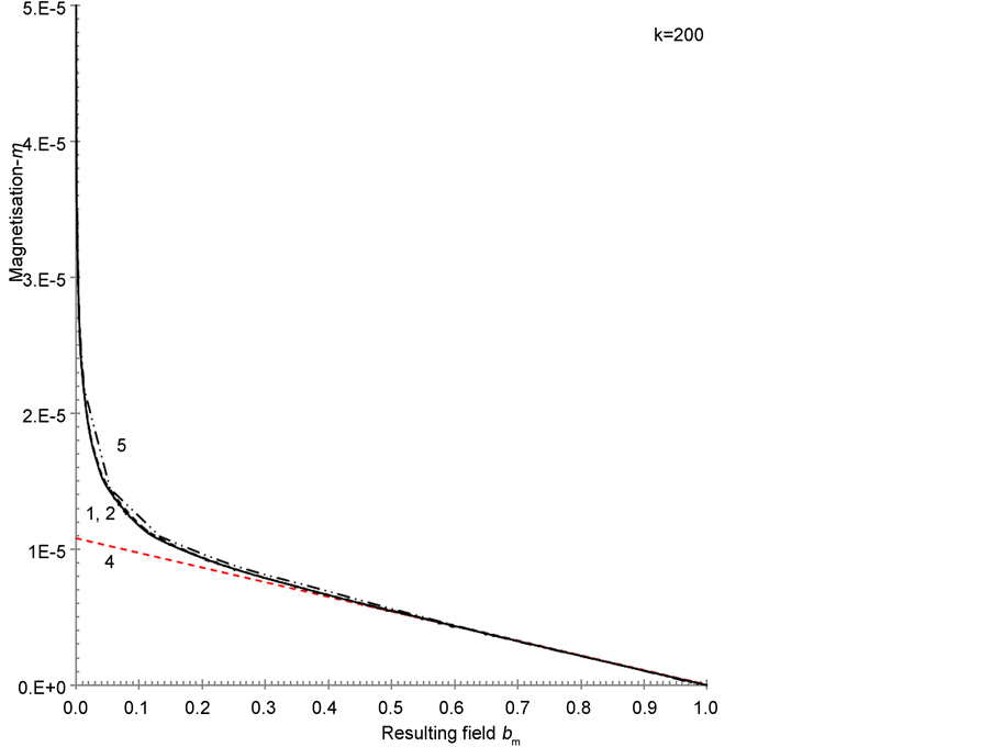
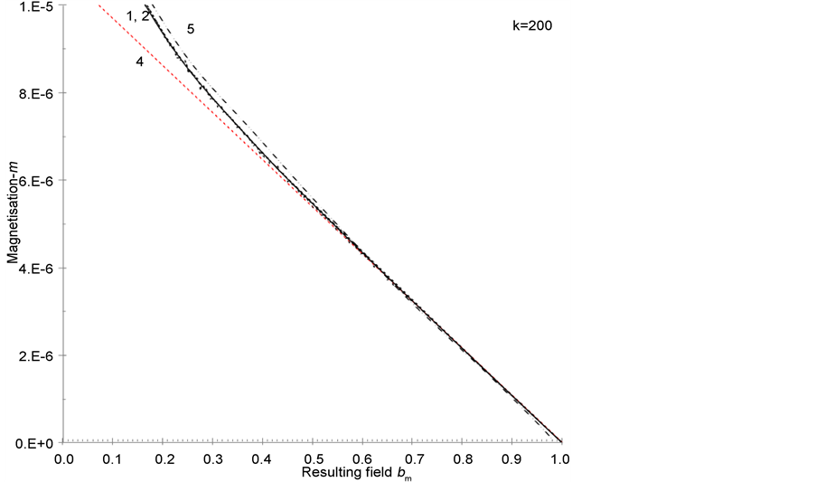
Figure 8. (a) Calculated for k = 100 magnetisation m as function of the field![]() : 1―as proposed here (m1); 2, 3―from the numerical solution, the dashed black line (m2) restored from [ [3] , Figure 7] and the dashed green line (m3) from the fit―[ [3] , Equation (19)]; 4―from Equation (27) (m4); 5―from [8] [9] [10] (dashed double dotted line, m5). The line numbering is the same as in Figure 5(a). (b) Calculated for k = 200 magnetisation m as function of the field
: 1―as proposed here (m1); 2, 3―from the numerical solution, the dashed black line (m2) restored from [ [3] , Figure 7] and the dashed green line (m3) from the fit―[ [3] , Equation (19)]; 4―from Equation (27) (m4); 5―from [8] [9] [10] (dashed double dotted line, m5). The line numbering is the same as in Figure 5(a). (b) Calculated for k = 200 magnetisation m as function of the field![]() : 1―as proposed here (m1); 2, 3―from the numerical solution, the dashed black line (m2) restored from [ [3] , Figure 7] and the dashed green line (m3) from the fit-[ [3] , Equation (19)]; 4―from Equation (27) (m4); 5―from [8] [9] [10] (dashed double dotted line, m5). The line numbering is the same as in Figure 5(a). (c) Fragment of the calculated for k = 200 magnetisation m as function of the field
: 1―as proposed here (m1); 2, 3―from the numerical solution, the dashed black line (m2) restored from [ [3] , Figure 7] and the dashed green line (m3) from the fit-[ [3] , Equation (19)]; 4―from Equation (27) (m4); 5―from [8] [9] [10] (dashed double dotted line, m5). The line numbering is the same as in Figure 5(a). (c) Fragment of the calculated for k = 200 magnetisation m as function of the field![]() , see Figure 8(b) for more. The line numbering is the same as in Figure 5(a).
, see Figure 8(b) for more. The line numbering is the same as in Figure 5(a).
this case). It is clear from the figure that m5 also fails to describe quantitatively the data represented by m1 (and m2): e.g., at ![]() the relative difference
the relative difference
![]() is 26.5%, which is not competitive and not what one expects after
is 26.5%, which is not competitive and not what one expects after
reading [8] [9] [10] .
5.2. Ginzburg-Landau Parameter ![]()
Representative for the range of ![]() (with
(with![]() , see [ [3] , Figure 1]) set of the magnetisation curves
, see [ [3] , Figure 1]) set of the magnetisation curves ![]() and
and ![]() is shown in Figure 5(b) and Figure 6(a) respectively.
is shown in Figure 5(b) and Figure 6(a) respectively.
In Figure 5(b) and Figure 6(a) the relative differences ![]() are below
are below
1.1% and 1.3% respectively in the entire range ![]() (except in the range:
(except in the range: ![]() where they are below 4% and 3.2% respectively, as further elaborated in Section 6.1). As expected [3] , the interpolation fit (m3) fails to de-
where they are below 4% and 3.2% respectively, as further elaborated in Section 6.1). As expected [3] , the interpolation fit (m3) fails to de-
scribe the data (m2) quantitatively, since k < 3 and thus ![]() is high. The
is high. The
data represented by m1 (and m2) are in good agreement with these represented by m4 at ![]() (so that both
(so that both ![]() and
and ![]() e.g., at
e.g., at ![]()
are below 0.4% (Figure 5(b)) and below 0.2% (Figure 6(a)), with ![]() and 0.75 respectively). It is clear from the figures that m5 fails to describe quantitatively the data represented by m1 (and m2): e.g., at b = 0.25 the relative dif-
and 0.75 respectively). It is clear from the figures that m5 fails to describe quantitatively the data represented by m1 (and m2): e.g., at b = 0.25 the relative dif-
ference ![]() is 24.5% (Figure 5(b)) and 16.1% (Figure 6(a)), which is not
is 24.5% (Figure 5(b)) and 16.1% (Figure 6(a)), which is not
competitive and not what one expects after reading [8] [9] [10] .
5.3. Ginzburg-Landau Parameter ![]()
Representative for the range of ![]() (with
(with![]() , see [ [3] , Figure 1]) set of the magnetisation curves
, see [ [3] , Figure 1]) set of the magnetisation curves ![]() and
and ![]() is shown in Figure 6(a) and Figure 6(b) respectively. In Figure 6(b) the relative difference
is shown in Figure 6(a) and Figure 6(b) respectively. In Figure 6(b) the relative difference
![]() is below 0.5% in the entire range of magnetic fields
is below 0.5% in the entire range of magnetic fields ![]()
(except in the range: ![]() where it is below 2% respectively, as further elaborated in section 6.1). As expected [3] the interpolation fit (m3) describes the
where it is below 2% respectively, as further elaborated in section 6.1). As expected [3] the interpolation fit (m3) describes the
data (m2) quantitatively, since k > 3 and thus ![]() is small, so both are
is small, so both are
represented by almost the same line in the figure. The data represented by m1 (and m2) are in good agreement with these represented by m4 at ![]() (so
(so
that both ![]() and
and ![]() e.g., at
e.g., at ![]() are below 0.3%, with
are below 0.3%, with
![]() ). It is clear from Figure 6(b) that m5 still fails to describe quantitatively the data represented by m1 (and m2): e.g., at
). It is clear from Figure 6(b) that m5 still fails to describe quantitatively the data represented by m1 (and m2): e.g., at ![]() the relative difference
the relative difference
![]() is 7%, which is not competitive and not what one expects after read-
is 7%, which is not competitive and not what one expects after read-
ing [8] [9] [10] .
5.4. Ginzburg-Landau Parameter ![]()
Representative for the range of ![]() (with
(with![]() , see [ [3] , Figure 1]) set of the magnetisation curves at
, see [ [3] , Figure 1]) set of the magnetisation curves at ![]() and
and ![]() is shown in Figure 6(b) and Figure 7(a) respectively. In Figure 7(a) the relative difference
is shown in Figure 6(b) and Figure 7(a) respectively. In Figure 7(a) the relative difference
![]() is below 1% in the entire range
is below 1% in the entire range ![]() (except in the range:
(except in the range:
![]() where it is below 1.3% respectively, as further elaborated in section 6.1). As expected the interpolation fit (m3) describes the data (m2) quantita-
where it is below 1.3% respectively, as further elaborated in section 6.1). As expected the interpolation fit (m3) describes the data (m2) quantita-
tively, since k > 3 and thus ![]() is small [3] so both are represented by
is small [3] so both are represented by
almost the same line in the figure. The data represented by m1 (and m2) are in good agreement with these represented by m4 at ![]() (so that both
(so that both
![]() and
and ![]() e.g., at
e.g., at ![]() are below 0.4%, with
are below 0.4%, with![]() ). It
). It
is clear from Figure 7(a) that m5 describes quantitatively the data represented by
m1 (and m2): with larger relative difference ![]() of e.g., 4% at b = 0.25 (as compared to
of e.g., 4% at b = 0.25 (as compared to![]() ) and with visible error in the magnetisation’s first deriv-
) and with visible error in the magnetisation’s first deriv-
ative (on![]() ).
).
5.5. Ginzburg-Landau Parameter ![]()
Representative for the range of ![]() (with
(with![]() ) set of the magnetisation curves at
) set of the magnetisation curves at ![]() and
and ![]() is shown in Figure 7(a)
is shown in Figure 7(a)
and Figure 7(b) respectively. In Figure 7(b) the relative difference ![]() is
is
below 0.6% in the entire range![]() . As expected the interpolation fit
. As expected the interpolation fit
(m3) describes the data (m2) quantitatively, since k > 3 and thus ![]() is
is
small [3] so both are represented by almost the same line in the figure. The data represented by m1 (and m2) are in good agreement with these represented by m4
at ![]() (so that both
(so that both ![]() and
and ![]() e.g., at
e.g., at ![]() are be-
are be-
low 0.5%, with![]() ). It is clear from Figure 7(a) that m5 describes quantitatively the data represented by m1 (and m2): with larger relative difference
). It is clear from Figure 7(a) that m5 describes quantitatively the data represented by m1 (and m2): with larger relative difference
![]() of e.g., 3% at b = 0.25 (as compared to
of e.g., 3% at b = 0.25 (as compared to![]() ) and the error in the
) and the error in the
magnetisation first derivative (on![]() ) is present.
) is present.
5.6. Ginzburg-Landau Parameter ![]()
Representative for the range of ![]() (with
(with
![]() ) set of the magnetisation curves at
) set of the magnetisation curves at ![]() and
and ![]() is shown in Figure 8(a) and Figure 8(b) respectively. Since the accurate numerical data for
is shown in Figure 8(a) and Figure 8(b) respectively. Since the accurate numerical data for ![]() are absent [3] , we use m3 instead of m2 in Fig-
are absent [3] , we use m3 instead of m2 in Fig-
ure 8(a). The relative difference ![]() is below 1% (Figure 8(a)) and
is below 1% (Figure 8(a)) and
![]() below 0.6% (Figure 8(b)) in the entire range
below 0.6% (Figure 8(b)) in the entire range![]() . The data
. The data
in Figure 8(a) represented by m1 (and m3) are in good agreement with these
represented by m4 at ![]() (so that both
(so that both ![]() and
and ![]() e.g.,
e.g.,
at ![]() are below 1%, with
are below 1%, with![]() ). The data in Figure 8(b) represented by m1 (and m2) are in good agreement with these represented by m4 at
). The data in Figure 8(b) represented by m1 (and m2) are in good agreement with these represented by m4 at
![]() (so that both
(so that both ![]() and
and ![]() e.g., at
e.g., at ![]() are below
are below
0.3%, with![]() ). It is clear from Figure 8(a) that m5 describes quantitatively
). It is clear from Figure 8(a) that m5 describes quantitatively
the data represented by m1 (and m3) with larger relative difference ![]() of e.g., 2% at b = 0.25 (as compared to
of e.g., 2% at b = 0.25 (as compared to![]() ) and the error in the magnetisa-
) and the error in the magnetisa-
tion 1st derivative (on![]() ) is present. It is clear from Figure 8(b) that m5 describes quantitatively the data represented by m1 (and m2) with larger relative
) is present. It is clear from Figure 8(b) that m5 describes quantitatively the data represented by m1 (and m2) with larger relative
difference ![]() of e.g., 4% at b = 0.25 (as compared to
of e.g., 4% at b = 0.25 (as compared to![]() ) and the
) and the
error in the magnetisation’s first derivative (on![]() ) is present.
) is present.
5.7. Ginzburg-Landau Parameter ![]()
The fragment of the magnetisation curve at k = 200 exemplifies that the error in the 1st derivative of the magnetization m5 is present at highest values of k and
results in the noticeable difference![]() . The noise of the magnetisation m2
. The noise of the magnetisation m2
caused by the digitalisation of the data [ [3] , Figure 7] is also visible in the figure.
To summarise, over the entire ranges of the GL parameter ![]() and of magnetic field
and of magnetic field ![]() excellent agreement between m1 and m2 is
excellent agreement between m1 and m2 is
achieved: the relative difference ![]() is below 1.5% everywhere (except at
is below 1.5% everywhere (except at
the narrow range: ![]() where it is below 4% as elaborated in section 6.1). This result validates the advanced symbolic approach of this paper. On the other hand, for the first time numerical results [3] for hexagonal and circular unit cells are accurately validated over the entire ranges of k and
where it is below 4% as elaborated in section 6.1). This result validates the advanced symbolic approach of this paper. On the other hand, for the first time numerical results [3] for hexagonal and circular unit cells are accurately validated over the entire ranges of k and ![]() in a transparent way with the (essentially independent) symbolic method of solving GL equations. Moreover, I find that the obtained close agreement of
in a transparent way with the (essentially independent) symbolic method of solving GL equations. Moreover, I find that the obtained close agreement of ![]() and
and ![]() makes some of the interpolation fits [ [3] , Equations (15)-(23)] obsolete. Clearly, the remaining discrepancy of
makes some of the interpolation fits [ [3] , Equations (15)-(23)] obsolete. Clearly, the remaining discrepancy of ![]() and
and ![]() can be reduced by expanding the data sets in Annex (the simplification error is now about 0.5%), making the direct comparison of the underlying data, revising the symbolic solution and the boundary conditions, etc. This however is beyond the scope of this paper. It must be noted, that magnetisation calculated from Equations (20)-(26) is rather sensitive to the errors in calculating the variational parameters. Therefore, in order to avoid the interpolation errors in calculating
can be reduced by expanding the data sets in Annex (the simplification error is now about 0.5%), making the direct comparison of the underlying data, revising the symbolic solution and the boundary conditions, etc. This however is beyond the scope of this paper. It must be noted, that magnetisation calculated from Equations (20)-(26) is rather sensitive to the errors in calculating the variational parameters. Therefore, in order to avoid the interpolation errors in calculating ![]() and
and ![]() (that can be caused e.g., by splines), values of
(that can be caused e.g., by splines), values of![]() ,
, ![]() and m are best calculated at exactly the same values of
and m are best calculated at exactly the same values of ![]() and k.
and k.
Presented in Annex data for the dependencies of ![]() and
and ![]() on k and
on k and ![]() contain the simplification error of up to 0.5% (caused by the limit in the size of the paper). I recommend that when aiming at the agreement better than 99% between magnetisation calculated symbolically and numerically, one has to use more accurate data obtained through the minimising the free energy density F of superconductor with respect to the variational parameters
contain the simplification error of up to 0.5% (caused by the limit in the size of the paper). I recommend that when aiming at the agreement better than 99% between magnetisation calculated symbolically and numerically, one has to use more accurate data obtained through the minimising the free energy density F of superconductor with respect to the variational parameters ![]() and
and![]() . Thus obviously “In order to achieve self-consistency in the theory the dependencies
. Thus obviously “In order to achieve self-consistency in the theory the dependencies ![]() and
and ![]() should be obtained by numerically minimising the function
should be obtained by numerically minimising the function ![]() with respect to
with respect to ![]() and
and![]() ” [8] [9] [10] , to which I add: the minimisation procedure is straightforward, use Equations (6) (7) (8), (16) (17) and a standard optimisation program, such as commonly available Solver in Excel. I find the quote above missing the “how” part (almost as to write: in order to get solution of GL equations, solve them).
” [8] [9] [10] , to which I add: the minimisation procedure is straightforward, use Equations (6) (7) (8), (16) (17) and a standard optimisation program, such as commonly available Solver in Excel. I find the quote above missing the “how” part (almost as to write: in order to get solution of GL equations, solve them).
6. The Critical Fields
6.1. The Lower Critical Field bc1
In this paper I calculate values of the field bc1 from Equations (25) (26) typically at![]() , since at
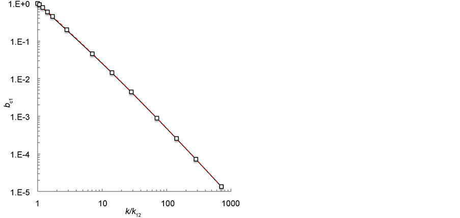
, since at ![]() the Equation (25) diverges. In Figure 9 the boxes show calculated this way dependence
the Equation (25) diverges. In Figure 9 the boxes show calculated this way dependence ![]() of the lower critical field bc1. The black solid line is calculated from the fit to the numerical results [3] [4] :
of the lower critical field bc1. The black solid line is calculated from the fit to the numerical results [3] [4] :
![]() (20)
(20)
with![]() ;
;![]() ;
;![]() ;
;![]() .
.
The red dashed line is calculated from the symbolic expression for isolated flux line [5] [6] :
![]() (32)
(32)
![]()
![]() (a) (b)
(a) (b)
Figure 9. Calculated dependence on k of the lower critical field bc1, (a): boxes―this paper (bc10); the solid black line―numerically, Equation (31) (bc12); the dashed line―Equation (32) (bc13); (b): fragment of the same, the black circles―the relative “error”, %:![]() .
.
In this range of k the bc1 changes by 5 orders of magnitude, so I find the agreement between![]() ,
, ![]() and
and ![]() reasonable (at k < 0 there is still room for improvement).
reasonable (at k < 0 there is still room for improvement).
6.2. The Upper Critical Field bc2
As noted [8] [9] [10] , and clear from Figures 5-8 and Annex, the value of the upper critical field ![]() following from the symbolic approach [8] [9] [10] is 1.5% lower than the true value of
following from the symbolic approach [8] [9] [10] is 1.5% lower than the true value of ![]() and therefore the correction is introduced in order to have the same upper critical point:
and therefore the correction is introduced in order to have the same upper critical point:
![]() (33)
(33)
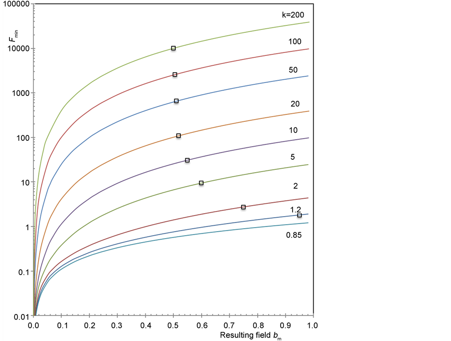
This correction is dealt with in section 4.2. Moreover, Figure 10 shows the values of Fmin, (derived from Equations (16) (17) through the minimisation procedure) corresponding to the data in Annex. The box on each curve corresponds to the value of magnetic field ![]() (Equation (29)), and separates the areas of validity for Equations (25) (26) and (27) valid respectively to the left or to the right from the box for any k > 1. Presented values of Fmin can be used as a reference when comparing different methods of solving GL equations.
(Equation (29)), and separates the areas of validity for Equations (25) (26) and (27) valid respectively to the left or to the right from the box for any k > 1. Presented values of Fmin can be used as a reference when comparing different methods of solving GL equations.
Finally, in order to illustrate the common feature of the ideal superconducting
![]()
Figure 10. Minimum value Fmin of the free energy density F (Equation (16) (17)) as function of the resulting magnetic field bm for the selected values of k (shown next to the corresponding lines).
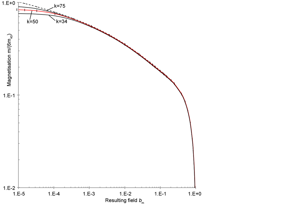
materials (in this case homogeneous, bulk, elliptically shaped, edge- and pin-free, placed in uniform magnetic field), in Figure 11 I show the magnetisation calculated for selected values of k = 34; 50 and 75 (typical for Nb3Sn; NbTi and REBCO respectively) and assuming vortex lattice with hexagonal unit cells. The solid lines represent m1 as proposed here; the dashed line ? m3 (interpolated from the fit [ [3] , Equation (19)]). The scaling factor m40 for the magnetisation in all cases is derived from Equation (28) (assuming![]() ), in addition to that the scaling factor of 6 is used in order to keep the magnetisation values below 1 in the figure. Scaled this way magnetic field dependence of the magnetisation for these very different materials in the field range
), in addition to that the scaling factor of 6 is used in order to keep the magnetisation values below 1 in the figure. Scaled this way magnetic field dependence of the magnetisation for these very different materials in the field range ![]() collapse practically at the same curve. At lower magnetic fields there is a stratification depending on the k value, besides m3 gives errors as expected [3] that are higher at lower k.
collapse practically at the same curve. At lower magnetic fields there is a stratification depending on the k value, besides m3 gives errors as expected [3] that are higher at lower k.
7. Conclusion
Known symbolic method [5] [6] [8] [9] [10] of solving Ginzburg-Landau equations has limited validity. Namely, assumed dependencies (interpolation fits) for the variational parameters ![]() and
and ![]() on the Ginzburg-Landau parameter k
on the Ginzburg-Landau parameter k
![]()
Figure 11. Calculated for k = 34, 50 and 75 magnetisation as function of the field![]() : the solid lines―m1 as proposed here; the dashed line―m3 (interpolated from the fit [ [3] , Equation (19)]). The scaling factor for the magnetisation in all cases is derived from Equation (28), in addition to that the scaling factor of 6 is used in order to keep the magnetisation ranging from 0.01 to 1 in the figure. The ±3% relative error (the vertical bars) is guide for an eye.
: the solid lines―m1 as proposed here; the dashed line―m3 (interpolated from the fit [ [3] , Equation (19)]). The scaling factor for the magnetisation in all cases is derived from Equation (28), in addition to that the scaling factor of 6 is used in order to keep the magnetisation ranging from 0.01 to 1 in the figure. The ±3% relative error (the vertical bars) is guide for an eye.
and on magnetic flux density ![]() are inaccurate and result in unacceptably high errors (reaching 25% and more). This limits applicability of otherwise excellent method. In the paper I eliminate several errors, extract and combine accurate symbolic solutions from the above and from [7] and provide for the first time precise dependencies for
are inaccurate and result in unacceptably high errors (reaching 25% and more). This limits applicability of otherwise excellent method. In the paper I eliminate several errors, extract and combine accurate symbolic solutions from the above and from [7] and provide for the first time precise dependencies for ![]() and
and ![]() on k and
on k and ![]() together with the simple and validated way of minimising the free energy density of superconductor. Resulting good agreement (98.5% for the entire range of magnetic flux density:
together with the simple and validated way of minimising the free energy density of superconductor. Resulting good agreement (98.5% for the entire range of magnetic flux density:
![]() and any value of the parameter
and any value of the parameter![]() ) between the advanced symbolic and the known numerical solutions of Ginzburg-Landau equations validates both and hopefully will result in wider use of the symbolic approach.
) between the advanced symbolic and the known numerical solutions of Ginzburg-Landau equations validates both and hopefully will result in wider use of the symbolic approach.
Acknowledgements
If you are interested to support this study, contact the author at:
o.a.chevtchenko@gmail.com. If you are interested in the results, contact us at: http://www.hts-powercables.nl. This research is funded privately and all rights belong to the author. Many thanks to A. A. Shevchenko for helping with difficult parts of this study, to R. Bakker for the inspirational atmosphere, to prof.-em. J. J. Smit for his support of this approach. A word of disgrace goes personally to Mr Jose Labastida, head of scientific department and to prof.-em. Helga Nowotny, former president of ERC, who chose to deny a funding for this study and thus created obstacles on the way to this result that could otherwise be published years earlier.
Cite this paper
Chevtchenko, O.A. (2017) Accurate Symbolic Solution of Ginzburg-Landau Equations in the Circular Cell Approximation by Variational Method: Magnetization of Ideal Type II Superconductor. Journal of Modern Physics, 8, 982-1011. https://doi.org/10.4236/jmp.2017.86062
References
- 1. Ginzburg, V.L. and Landau, L.D. (1950) Towards the Superconductivity Theory. Journal of Experimental and Theoretical Physics, 20, 1064.
- 2. Bardeen, J., Cooper, L.N. and Schrieffer, J.R. (1957) Microscopic Theory of Superconductivity. Physical Review, 106, 162.
- 3. Brandt, E.H. (2003) Properties of the Ideal Ginzburg-Landau Vortex Lattice. Physical Review B, 68, Article ID: 054506.
- 4. Brandt, E.H. (2012) Mixed State Properties. In: Rogalla, H. and Kees, P., Eds., 100 Years of Superconductivity, Taylor & Francis Group, Abingdon-on-Thames, 125-137.
- 5. Clem, J.R. (1975) Simple Model for the Vortex Core in a Type II Superconductor. Journal of Low Temperature Physics, 18, 427.
- 6. Hao, Z. (1991) Model for the Reversible Magnetization of High-[Kappa] Type-II Superconductors: Application to High-Temperature Superconductors. PhD Book, Iowa State University, Ames.
- 7. Abrikosov, A.A. (1957) On the Magnetic Properties of Superconductors of the Second Group. Journal of Experimental and Theoretical Physics, 5, 1174.
- 8. Pogosov, V.V., Rakhmanov, A.L. and Kugel, K.I. (2000) Magnetization of Type-II Superconductors. Journal of Experimental and Theoretical Physics, 19, 588.
- 9. Pogosov, V.V., Kugel, K.I., Rakhmanov, A.L. and Brandt, E.H. (2001) Approximate Ginzburg-Landau Solution for the Regular Flux-Line Lattice. Circular Cell Method. Physical Review B, 64, Article ID: 064517.
- 10. Pogosov, V.V. (2002) Влияние поверхности и размеров образца на структуру смешанного состояния сверхпроводников второго рода. PhD Book, Moscow. (In Russian)
- 11. Chevtchenko, O.A., Smit, J.J., de Vries, D.J. and de Pont, F.W.A. (2014) Modelling of Magnetisation and Intrinsic Properties of Ideal Type II Superconductor in External Magnetic Field. Proceedings of the 2014 COMSOL Conference, Cambridge.
https://www.comsol.com/paper/download/199917/chevtchenko_paper.pdf
- 12. Alstrøm, T.S., Sørensen, M.P., Pedersen, N.F. and Madsen, S. (2011) Magnetic Flux Lines in Complex Geometry Type-II Superconductors Studied by the Time Dependent Ginzburg-Landau Equation. Acta Applied Mathematics, 115, 63.
https://doi.org/10.1007/s10440-010-9580-8
- 13. Saint-James, D., Sarma, G. and Thomas, E.J. (1969) Type II Superconductivity. Elsevier Science & Technology.
Annex
Accurate dependencies of the variational parameters ![]() and
and ![]() obtained from the minimising the free energy density F, see Equations (16) (17) (Tables A1-A4). The dimensional and dimensionless quantities and scaling factors (Table A5).
obtained from the minimising the free energy density F, see Equations (16) (17) (Tables A1-A4). The dimensional and dimensionless quantities and scaling factors (Table A5).
Note that in order to simplify comparisons with [8] [9] [10] in Tables A1-A4 the values of ![]() are not corrected (by 0.985).
are not corrected (by 0.985).
![]()
Table A1. Spline data for the calculated variational parameter ![]() at
at![]() .
.
![]()
Table A2. Spline data for the calculated variational parameter ![]() at
at![]() .
.
![]()
Table A3. Spline data for the calculated variational parameter ![]() at
at![]() .
.
![]()
Table A4. Spline data for the calculated variational parameter ![]() at
at![]() .
.
*same values as in Table A2 are given here for convenience.
![]()
Table A5. The dimensional and dimensionless quantities and scaling factors.


 , which is good basis for many engineering applications. As a result, a theoretical tool is developed using known symbolic solutions of GL equations with accuracy surpassing that of any other known symbolic solution and approaching that of numerical one.
 with λ, ξ London penetration depth and the coherence length respectively. Moreover, the magnetic field dependence of (reversible) magnetisation can be calculated in seconds.
 , which is sufficient for many engineering applications.
 so that both Bc2 and
  are defined through
  and Annex provides more details. Below there are six mean (averaged over the unit cell area) magnetic field magnitudes (magnetic flux densities) in use: thermodynamic (equilibrium, applied) field Ba, magnetisation M (from the induced currents), the resulting (total) field:
 with the local field br defined by GL equations in Table 1;
 respectively. Furthermore, in this paper
  is considered
 is magnetic flux quantum. Note the local magnetic flux density
 introduced (along with the four other local quantities) in Table 1 and Section 2.4. Here and below I use the dimensionless units: distance r, modulus of the magnetic vector potential
 , modulus of the super-velocity
 ,
, and
and , current density
 , magnetic flux quantum


