Journal of Modern Physics
Vol.3 No.2(2012), Article ID:17698,13 pages DOI:10.4236/jmp.2012.32026
Classical Interpretations of Relativistic Phenomena
Indian Physical Society, Calcutta, India
Email: sankarhajra@yahoo.com
Received October 9, 2011; revised December 16, 2011; accepted January 4, 2012
Keywords: Electromagnetic Entities; Electromagnetic Mass; Gravitation; Old Physics; Special Relativity; General Relativity
ABSTRACT
Electric charges, electric & magnetic fields and electromagnetic energy possess momentum and energy which we could experience with our sense organs. Therefore, all these are real physical entities (objects). All physical objects are subject to gravitation. Therefore, electromagnetic entities should similarly be subject to gravitation. In this paper, we have shown that classical physics with this simple consideration is equivalent to the theory of relativity—special & general— to explain many puzzling electrodynamic as well as gravitational phenomena.
1. Introduction
Important observations on the behavior of light waves began to be performed from the time of Roemer (1670) and important experiments on electricity and magnetism began to be conducted from the time of Coulomb (1783). Maxwell (1865) tried to unify both streams of knowledge and dared to realize what light was. There were numerous experiments to demonstrate that Maxwell’s theory was correct, though some might argue that the theory was inadequate.
In the Maxwell’s theory, if c is considered to be the speed of light in free space, Maxwell’s equations are then valid in free space where the earth is obviously moving with an appreciable velocity. Therefore, the Maxwell’s equations should be affected on the surface of the moving earth. But curiously, all electromagnetic phenomena as observed on the surface of the moving earth are independent of the movement of this planet. To dissolve this problem, Einstein (1905) assumes that Maxwell’s equations are invariant to all observers in steady motion which acts as the foundation of Special Relativity. In the second place, the relativistic mass formula is routinely confirmed in particle accelerators. Therefore, Special Relativity is held to be more acceptable than Classical Electrodynamics. In the second decade of the past century, Einstein extended his special relativity to General relativity, a spacetime curvature physics wherein he explained many puzzling gravitational phenomena with the application of his space-time curvature proposition.
From the days of inception of the theory of relativity (1905), numerous physicists like Paul Ehrenfest (1909), Ludwig Silberstein (1920), Philipp Lenard (1920), Herbert Dingle (1950), F. R. Tangherlini (1968), T. G. Barnes et al. (1976), R. Tian & Z. Li (1990) and many others have doubted (fully or partially) over the foundation of the theory of relativity and many of them have proposed alternative approaches. In the period between the last decade of the last century and the first decade of the present century (1991-2010), C. A. Zapffe, Paul Marmet, A. G. Kelly, N. Hamdan, R. Honig and many others have made important contributions in this direction.
In the first part of this paper, we have shown that the mass of a point charge as per Classical Electrodynamics is the same as that of Special Relativity and the foundation of both the deductions lies in Classical Electrodynamics of Heaviside (1988). Therefore, mass formula confirmed by the particle accelerators is fully consistent with Classical Electrodynamics too.
In the second part, we have shown that the consideration of the effects of gravitational field of the earth on electromagnetic entities easily explains classically those puzzling gravitational phenomena (explained by Einstein) as well as why all electromagnetic phenomena as observed on earth’s surface are independent of the movement of the earth; and this elucidates that both the invariant proposition and the space-time curvature proposition of Einstein are unnecessary.
Our goal is to show here the efficacy of the classical physics to interpret relativistic phenomena rationally and easily. In this study we have only used Maxwell’s electromagnetic equations, Newton’s equations of motions and his theory of gravitation. We have used no theory of our own.
2. Classical Electrodynamics—Auxiliary Potentials & Auxiliary Fields
2.1. The Electric Field (E) and the Induced Magnetic Field (B*) of a Steadily Moving System of Charges
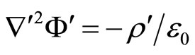
The potential  of a stationary system of charges is determined by the Poisson’s equation:
 (1)
(1)
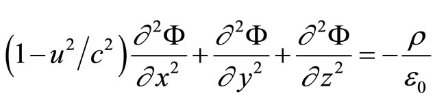
But, the scalar potential ( ) and the induced vector potential (
 ) of this system of charges when moves in the OX direction with a velocity
  are governed by D’Alembert’s equation:
 (2)
(2)
 (3)
(3)
where  is the charge density of the system,
  is the permittivity and
 is the permeability of free space such that
  and
and  are the Cartesian co-ordinates introduced in free space.
In such a situation, the potentials at the point  at the instant t and the potentials at the point
 at the instant
  in free space will be the same. Therefore,
 (4)
(4)
 (5)
(5)
Similarly,
 (6)
(6)
Equations (5) & (6) are steady state equations in Classical Electrodynamics.
By the use of Equation (5), Equation (2) could be replaced by
 (7)
(7)
and by the use of Equation (6), Equation (3) should be replaced by
 (8)
(8)
 (9)
(9)
Comparing Equation (7) with Equation (8), we have,
 (10)
(10)
Therefore, to determine  and B* we are only to determine
 .
.
Heaviside first published the deductions of B* and  through A* directly by the use of his operational calculus in 1888 [1] and then in 1889 [2]. Thomson [3] & Lorentz [4] however, traveled a different path and solved the problem in a beautiful way which is as follows:
Now, construct an auxiliary system  where the charged system is considered stationary such that
 (11)
(11)
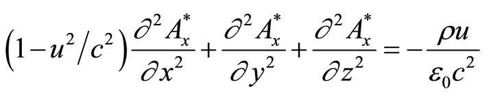
which transforms Equation (7) to
 (12)
(12)
Since this equation is used to determine the potential of a stationary system of charges as in Equation (1), the problem is reduced to an ordinary problem of electrostatics.
The auxiliary system constructed by Equations (11) is static and elongated. There, we have,
 (13)
(13)
 (14)
(14)
where  is the auxiliary charge density and
  is the auxiliary scalar potential or the mathematical auxiliary of
 .
.
Constructions of auxiliary quantities for point charge electrodynamics are very simple as shown in the Section 2.7, as the shape of the point charge is considered to be the same in the auxiliary system. But to deduce auxiliary quantities related with large charge electrodynamics is very difficult as large charges change their shapes in the auxiliary system, which requires separate independent treatment.
2.2. Relation between Real Scalar Potential (for a Steadily Moving System of Charges) and Auxiliary Scalar Potential
Comparing Equation (12) with Equation (14) using Equation (13), we have,
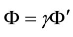 (15)
(15)
Thus we see that the potential of a moving system of charges is not connected to the potential of the same system at rest. That potential is related with the potential of the stationary system (auxiliary system) in which all the co-ordinates parallel to OX, OY and OZ have been changed in the ratio determined by Equation (11).
From the above analysis, we have,
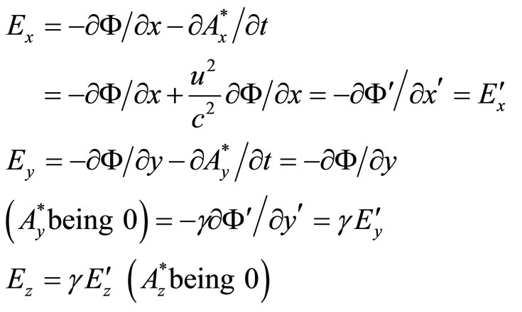 (16)
(16)
 ,
,  and
and  represent mathematical auxiliaries of the field components
 ,
,  ,
, 
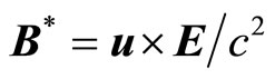
From 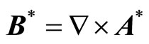 and Equations (9), (10) and (16), we have for the induced magnetic field
 :
:
 (17)
(17)
From which we get,
 (18)
(18)
2.3. The Magnetic Field (B) and the Induced Electric Field (E) of a Steadily Moving System Containing Line Current
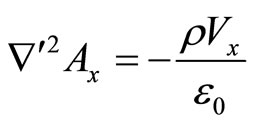
The vector potential  of a line current (flowing in any arbitrary direction) moving with a system with constant velocity of translation
  is as well known governed by the equation,
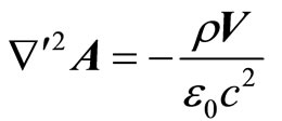 (19)
(19)
where  is the current density.
  represents the velocity of charges (constituting the line current) with respect to free space when the system moves with a velocity
  in free space in the OX direction.
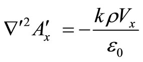
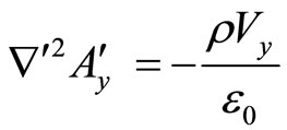
Using auxiliary Equation (11), in a similar procedure used for the construction of Equation (12), we have from Equation (19),
 (20)
(20)
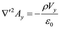 (21)
(21)
and the similar equation for the z-component.
For the auxiliary system when the magnetic field depends on the length of the current element but not on its cross-section as in the case of a line current, we have from a similar procedure used for the construction of Equation (14),
 (22)
(22)
 (23)
(23)
and the similar equation for the z'-component ( ,
, and
and  are the components of the Auxiliary magnetic potential in the auxiliary elongated system).
2.4. Relation between Real Vector Potential (of a Moving System of Current) and Auxiliary Vector Potential
By comparison of Equations (20), (21) and the similar Equation for  -component with the relevant equations in the auxiliary system i.e., Equations (22), (23) and the similar equations for the
  -component we have,
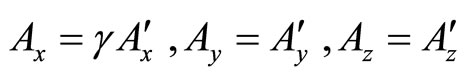 (24)
(24)
whence, by using , for the moving line current, we have, for the original vector field
 (25)
(25)
For the induced electric field governed by the relation
we have,
 (26)
(26)
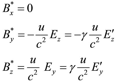
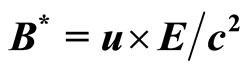
Now, when a system with an independent electric field (originating from charges of any shape and size) and an independent magnetic field (originating from line currents flowing within the system in any arbitrary directions) is steadily moving with a velocity  in the OX direction, we get the following relations [adding the same components of fields together as in Equations (16) and (17) with Equations (25), and (26).
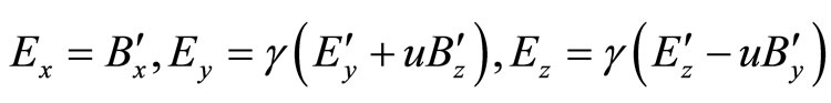 (27)
(27)
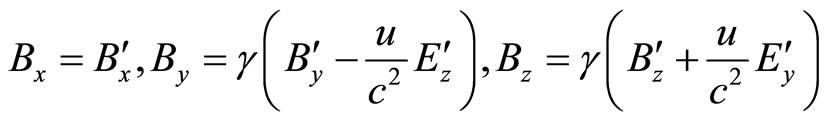 (28)
(28)
2.5. Velocity of Light in a Dielectric Steadily Moving in Free Space: Fresnel Drag Coefficient in Fizeau Experiment
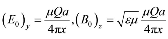
Let a point charge  at the time t pass the origin of a Cartesian co-ordinate system constructed in free space. Let the charge have acceleration a in the negative direction of the OY axis. Then from Maxwell, a spherical wave will radiate from the origin as it were a point source with the field vectors as function of time and distance from the source. Now let this radiation pass through a piece of stationary dielectric (refractive index n) that touches the origin of the radiation. Now let us concentrate on the propagation of the wave along OX direction in the dielectric. We have now from Maxwell,
 (29)
(29)
as per previous discussion the auxiliary fields will be
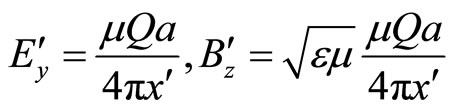 (30)
(30)
[ , the permeability,
  the permittivity of the dielectric,
  and
and  where
where  for the dielectric].
For, the fields owe their origins from point charges and the fields are manifested in the dielectric.
Therefore, from Equations (29) and (30),
 (31)
(31)
Now if the dielectric moves with a velocity  in free space in OX direction, the electric field inside the dielectric will change to
  and the magnetic field inside the dielectric will change to
  and thereby the velocity of the ray in the dielectric will change to
  such that using Equations (27) & (28) as modified for dielectric, we get,
 (32)
(32)
Now dividing the numerator and the denominator by  and using Equation (31) we have,
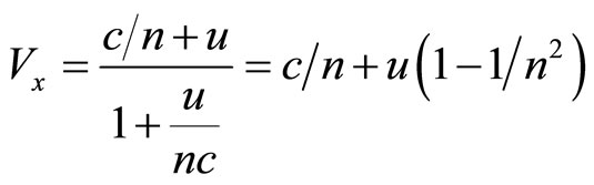 (33)
(33)
(vide alternative deduction in [5]).
2.6. Velocity of a Charge in a Steadily Moving Electromagnetic System
Let a system of charges and currents be stationary in free space represented by Cartesian Coordinates. Now let a point charge q placed inside the system move with an instanttaneous velocity  in the OX direction due to an electric field (E0) and a magnetic field (B0) originating from those charges and currents.
Then the y-component of the Lorentz force acting on q should be zero, i.e.,
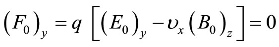 (34)
(34)
from which we get,
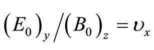 (35)
(35)
For a steady motion of the point charge with that velocity for all the time, we are to construct the following field equations from an analogy of the fields as given in Equation (30):
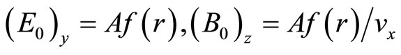 (36)
(36)
where A is a constant and the origin of the fields are point charges.
The relevant auxiliary fields are
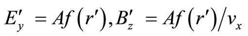 (37)
(37)
In that case, we have,
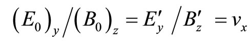 (38)
(38)
Now, if the system moves with a velocity u in the OX direction in free space, we have for the velocity  of the test charge in the free space using Equations (27) & (28),
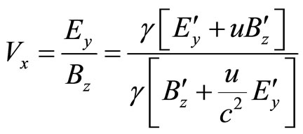 (39)
(39)
where  and
and  are the electric and magnetic fields due to the system of charges and currents moving with the system.
Dividing the numerator and the denominator by  and using Equation (38) we have,
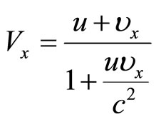 (40)
(40)
when the test charge moves in any arbitrary direction in XY plane, we have (say),
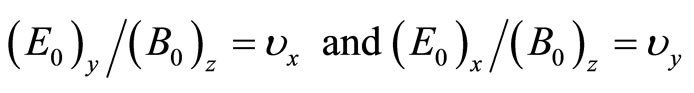 (41)
(41)
Now, if the system moves with a velocity u in free space in the OX direction [using Equations (27) and (28)]
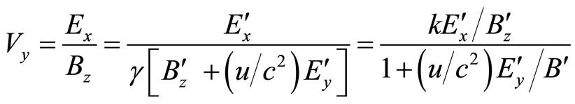 (42)
(42)
For steady motion we have  as in Equation (41) and therefore, following arguments as given to construct Equation (38), we have,
 (43)
(43)
Now using Equations (38) & (43), we get from Equation (42),
 (44)
(44)
and similarly,
 (45)
(45)
2.7. Derivation of the E-Field and the B-Field and Electromagnetic Momentum of a Steadily Moving Point Charge
Now suppose that a point charge moving with a velocity u in the OX direction passes the origin of a co-ordinate system fixed with the free space at the instant t.
We are to determine E at P  at the instant t.
The auxiliary fields should be in the same form as those of the stationary fields with the auxiliary co-ordinate notations (as a point charge is a point charge in the auxiliary system).
 (46)
(46)
where  are the components of auxiliary electric field at
 which is the corresponding point of P
 such that the angle between OX and OP is
  whence using Equations (11) and (16), we have,
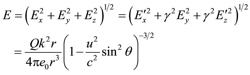 (47)
(47)
The auxiliary  is directed along
  (
( ). Therefore, the real field
  is directed along
  (
( ). Now, remembering Equation (18) we have,
 (48)
(48)
These deductions could be found in the works of Morton [6], Whittaker [7], and Oppenheimer [8]. Miller’s [9] comments in this respect is noteworthy. The similar results were derived by Liénard-Wichert [10,11] from the consideration of retarded potential. Many authors as cited by Jefimenko [12] derive the results classically either from the consideration of retarded potentials or from generalised time dependent Biot-Savart and Coulomb field laws. Heaviside first derived Equations (47) & (48) as early as in 1888. Therefore, these fields are called Heaviside’s fields. The deductions of Special Relativity are the same as the deduction given above. Special relativity assumes that the auxiliary equations are real which does not affect this deduction in case of a point charge.
It could easily be shown by the similar analysis that a steadily moving charged ellipsoid having the axes 
 (Heaviside’s Ellipsoid,
 ) has the same external effects as those of a similarly moving point charge as the ellipsoid is a sphere in an auxiliary system, and the sphere has the same form of potential as that of a point charge in the stationary system. This important observation was first noted by Oliver Heaviside [13].
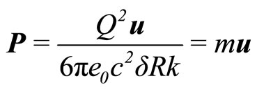
Electromagnetic Momentum (P) of a point charge moving with a velocity u in the OX direction,
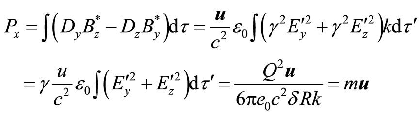 (49)
(49)
(as ,
,  and
and  are related to a sphere and so each integral is equal to
 )
)
where
 (50)
(50)
and
 (51)
(51)
In this instant case,  ,
, .
.
 (52)
(52)
Suppose that a point charge at rest in the free space is subjected to a force F which displaces the charge a distance dx and thereby, the charge attains a velocity u in the free space. In that case, we could classically deduce from Equation (52), the kinetic energy K of that point charge as (when u = c),
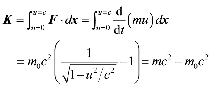 (53)
(53)
The equation is applicable only to a point charge but not to a big charge or a point particle.
This Equation (49) defines the longitudinal electromagnetic force,
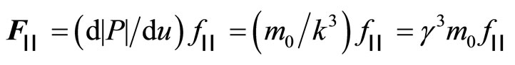 (54)
(54)
where F and f (acceleration of the point charge) are parallel to u.
and the transverse electromagnetic force
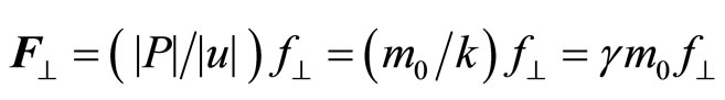 (55)
(55)
where f is parallel to F and perpendicular to u.
The quantities  and
and 
 are respectively called the longitudinal and transverse electromagnetic masses of a steadily moving point charge.
2.8. Electromagnetic Fields and the Ulhenbeck-Goudsmit Precession
Electromagnetic momentum of a point charge possesses  coefficient. This coefficient should be responsible for the spinning of a spherical electron with an appreciable radius while it moves in its orbit.
We know from Faraday that when a system of charges moves with a velocity u in free space, a magnetic field
 (56)
(56)
is induced in a small conducting strip stationary in the free space (E being the electric field in the stationary conductor due to the system of moving charges).
Faraday also observes that if the system of charges be stationary in the free space and the strip moves with the same velocity u in the free space in the same direction a magnetic field
 (57)
(57)
is induced in the conductor.
Now if a spherical rigid electron with an appreciable radius is embedded in the moving strip and the strip moves in an electric field, there will be a magnetic field inside the strip and then from the consideration of Ulhenbeck and Goudsmit, the electron will precess about its instantaneous normal to the orbital plane with the angular velocity
 (58)
(58)
e is the charge of the electron and m is defined as per the Equation (51).
When the electron rotates in a circular orbit of radius r with the velocity u in a Coulomb field in the anticlockwise direction, we have,
 (59)
(59)
Using the Equation (59), and the well known relation  we could get from Equation (58),
 (60)
(60)
where  is the angular velocity of the electron in its orbit.
We see here that Ulhenbeck-Goudsmit precession is in the anticlockwise direction when the electron moves in its orbit in the anticlockwise direction.
2.9. Electromagnetic Momentum and the Thomas Precession
Apart from this hypothetical Ulhenbeck-Goudsmit precession of the electron, the electron should spin around its own axis while it moves in its orbit from the consideration of classical electrodynamics of Maxwell.
The expression for electromagnetic momentum of a steadily moving point charge contains a  coefficient.
In case of a curved motion of a spherical rigid electron there is always a difference of the  coefficients of the x-component and y-component of the electromagnetic momentum [cf. Equation (52)] of the infinitesimal charge element on any point
  on the body of the electron moving in a curved path and this gives rise to the spin of the electron responsible for Thomas Precession.
To get a picturesque view of this interesting phenomenon, let us consider that this paper plane represent any plane of the free space. Let us now construct a Cartesian Co-ordinate system OX and OY at any point O in this paper plane (Figure 1) and let the centre of the electron be pivoted in this paper plane in such a way that the circumference of the electron normal to its axis is coplanar with this paper plane. Now let the centre of the electron be moved from O to P in the curved path OP during a time period . Let for simplicity consider that the centre of curvature of the curved path OP lie on OY.
In this set-up, we shall view the curved motion of the electron and calculate the spinning of electron roughly. Consider that the electron starts its motion from O with a velocity u towards OX and after a small time interval  it reaches A. When it reaches A, the electron is pushed with such a (very small) velocity
  towards a direction parallel to OY so that the electron will reach the point P after the time interval
 .
.
Therefore,
 (61)
(61)
The angle  being very small we have,
 (62)
(62)
Now the x-component and the y-component of the electromagnetic momentum of the infinitesimal charge element around any point  on the electron body which is moving with the centre of the electron,
 (63)
(63)
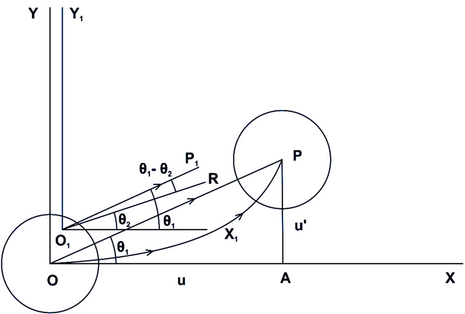
Figure 1. Curved motion of an electron and consequent Thomas precession as per Maxwell.
 (64)
(64)
(u being large and  being very small) where
  is the electromagnetic mass of that infinitesimal charge element at rest in free space as defined in Equation (50).
Therefore, the resultant direction of momentum ( ) of that infinitesimal charge element at
  will roughly make an angle
  with
with  axis drawn parallel to OX at
  such that
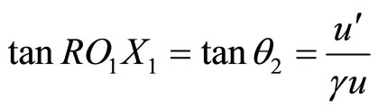 (65)
(65)
 being small, we have,
 . (66)
But, the charge element at  should normally move with its centre towards
  parallel to OP such that
 (67)
(67)
Under this situation, the point  should deflect towards
  axis (parallel to OX axis).
The angle of deflection of the direction of motion of the moving infinitesimal charge element around  towards
  axis (parallel to OX axis)
 (68)
(68)
Thus during the travel of the electron in the anticlockwise direction in its orbit for the time period , every infinitesimal charge element of the electron body will tend to deflect by a very small angle
  in the clockwise direction.
But the electron is a rigid body and pivoted, too, to a fixed circular path. Therefore, during the time period , the electron will rotate through an angle
  in the clockwise direction and as the electron moves always in a curved path, this rotation continues.
Now at the point P, the velocity components of the centre of the electron read:
 (69)
(69)
 (70)
(70)
 being the angle that the arc OP subtends at the centre (not shown in the Figure 1),
  , the radius of curvature of OP and
  being the angular velocity of the electron in its orbit.
From Equations (69) and (70), we get,
 (71)
(71)
Using Equation (71), we get from Equation (68),
 (72)
(72)
 (73)
(73)
 being the angular velocity of spinning of the electron around its axis while it moves in its orbit.
We see that this spinning (Thomas spinning) is in the clockwise direction when the electron rotates in its orbit in the anticlockwise direction.
The Equation (73) could be written using Equation (59) as
 (74)
(74)
Net Precession.
Therefore, the net angular velocity of precession could be roughly determined as
 (75)
(75)
We see that the net precession is in the anticlockwise direction.
Alternatively, using Equations (58) & (74) this could be written as
 (76)
(76)
Thus when an electron rotates in its orbit in the anticlockwise direction, the net precession is in the anticlockwise direction.
2.10. Transverse Doppler’s Effect
As per classical electrodynamics, an elastic electromagnetic force acting on point charges inside matter causes electromagnetic radiation. Now if the matter moves, the dipole moves with it. Thereby the electromagnetic force inside matter changes and consequently, frequency and time-period of oscillation of the dipole change as per the following classical equations.
Let an electric force F0 (originating from a small charge) drive a point charge back and forth from one end to the other end of a radiating dipole stationary in free space. Then, as per classical equation,
 (77)
(77)
velocity of oscillation being small, where  is the electromagnetic mass of the charge in the stationary dipole,
  is the radian frequency of oscillation of the charge, S is the separating distance of the dipole.
Now, if the dipole moves with a velocity u in free space in any direction perpendicular to its direction of oscillations, the electric force and the magnetic force acting on the charge will be respectively from Equations (47) and (48), (when  = 90˚)
  and
and . Therefore, total electromagnetic force acting on the moving charge is
 (78)
(78)
Now, when the above dipole moves and radiates, we have,
 (79)
(79)
where  is the transverse electromagnetic mass of the charge in the moving dipole as defined by the Equation (55),
  is the frequency of oscillation of the charge which is moving with a velocity u in free space with the dipole and F is the electromagnetic force acting on the moving charge.
Comparing Equations (77) and (79) using Equations (55) and (78) for the dipole moving with an uniform velocity in any direction perpendicular to its direction of oscillation we have,
 (80)
(80)
The equation explains transverse Doppler’s effect classically.
2.11. The So-Called Time Dilation
Now if the frequency changes, time period too changes.
For a radiating dipole stationary in free space,
 (81)
(81)
where  is the oscillation period and
  is the radian frequency. If the same radiating dipole moves with a velocity
  in free space in a direction perpendicular to its direction of oscillation, then for the moving dipole the oscillation period
  and radian frequency
  satisfy,
 (82)
(82)
Comparing Equations (81) with (82) using Equation (80) we have,
 (83)
(83)
or the period of oscillation of the above moving dipole increases with its velocity in free space.
2.12. Increment of Life Spans of Moving Radioactive Particles
A radioactive particle decays when electric and magnetic forces inside the particle act to disintegrate the particle. When the radioactive particle moves, the electric and magnetic forces acting inside the particle change. And consequently, the disintegration process in the moving radioactive particle changes as per the following classical equations:
Let at the initial instant , there be
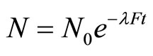
  radioactive particles of a particular species. Let us find the number N of those particles that will remain untransformed by an arbitrary time
 . Since we are dealing with spontaneous transformation, we may presume that the rate at which the total quantity of radioactive particles is diminishing at any instant is 1) proportional to the total quantity N of radioactive particles present at that instant when the magnitude of the electromagnetic force
  (acting inside the particles on the charge to be detached) is constant, and 2) proportional to the magnitude of the electromagnetic force
  acting inside the particles on the charge to be detached when N is constant, which may be a priori plausible. Therefore we may write:
 (84)
(84)
where  and N both vary. Moreover, we have,
 (85)
(85)
Combining above two equations we have,
 (86)
(86)
where  is the proportionality constant.
Now if the radioactive particles move with a velocity u in free space in any direction perpendicular to their direction of the detaching force, after a time t we will find N untransformed particles such that
 (87)
(87)
where  is the magnitude of force acting on the charge to be detached in the moving particle. Comparing Equations (86) with (87) using Equation (78), we have,
 (88)
(88)
This analysis at once destroys “here is one time”, “there is another time”—concept as well as the twin paradox of relativity.
Now, if the source be stationary in the free space and the observer moves, from the consideration of Maxwell, there should be no transverse Doppler effect and no time increment. If transverse Doppler effect and time increment are confirmed experimentally in such cases (with electromagnetic corrections), only then some special theories could be held superior in this regard.
Some particles like Lambda particles originate when a charged particle collides with a charged particle and on decay they produce charged offspring. Though these particles are outwardly neutral, they are not neutral in its interior. Therefore, when in steady motion, life spans of lambda like particles should increase with velocity by  factor.
3. Interaction of Electromagnetic Entities with Gravitation
3.1. Electric Charge and Gravitation
We know that electric charges possess momentum and energy just like all other physical objects. We could experience momentum and energy of these charges with our sense organs. Therefore, charges are real physical entities (objects). All objects are subject to gravitation and they have the same acceleration towards the centre of gravity in the same gravitating field. Therefore, charges should similarly be subject to gravitation and the acceleration of a point charge should be the same as the acceleration of a point object and that should be directed towards the interacting gravitating field (unlike its acceleration during its interaction with the electric field).
This implies that the gravitating mass of a point charge is proportional to its longitudinal electromagnetic mass. Transverse electromagnetic mass should have no role in this interaction. If it had any role in the interaction, charges should not have the same acceleration as those of the material bodies in the same gravitating fields. Thus, in a gravitating field, a point charge acts a mass point; mass of the mass point is proportional to the longitudinal electromagnetic mass of the point charge.
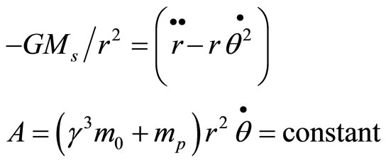
Thus, when a point charge moves in a gravitating field, by dint of our above analysis, we have for the Radial force:
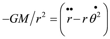 (89)
(89)
where G is the gravitational constant, M is the total mass (non-electromagnetic mass & mass originating from charges in the gravitating body) of the gravitating body concentrated at the origin and the point charge passes the point ( ) in the plane of motion in the polar co-ordinate.
Now, as per the old physics, Cross-radial Force:
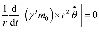 (90)
(90)
From which we have the angular momentum of the point charge,
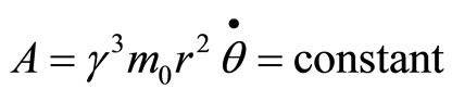 (91)
(91)
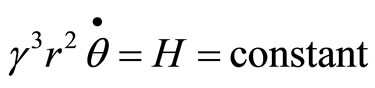 (92)
(92)
Now let
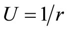 (93)
(93)
Therefore, the equation of motion of the point charge in a gravitating field should be as per Newtonian analysis:
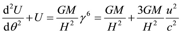 (94)
(94)
[replacing H of the second term of the last expression by Equation (92) and noting that for circular motion  ].
].
 (95)
(95)
Vide full calculations in [14,15].
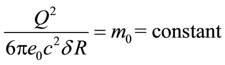
3.2. Exact Equation of Planetary Motion
Suppose that a planet of non-electromagnetic mass  originating from
  amount of positive and negative charges in total (ignoring the sign of the charges). For simple calculation let us assume that the positive and negative charges are concentrated separately near the centre of the planet. Let
  be the total mass (non electromagnetic mass & mass originating from the charges associated with the sun). In this situation as per the previous discussion, the equation of planetary motion will be as under:
 (96)
(96)
when  and m0
 ,
,
 (97)
(97)
 (98)
(98)
Therefore, the equation of motion of a planet in the sun’s gravitating field should be
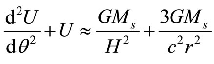 (99)
(99)
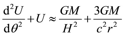
The Equation (99) is similar to Equation (95), This classical equation will at once explain the advance of the perihelion Mercury.
Vide full calculations in [14,15].
3.3. Equation of Motion of the Light Rays in the Gravitating Field of the Sun
Light-rays possess electromagnetic momentum and electromagnetic energy. Many people believe that an electron and a positron “coming together, could annihilate each other with the emission of light or gamma rays” [16] and “light also acts like electrons” [17]. If that be so, a point light will similarly be subject to gravitation as in the case of a point charge. But in this case,  for a point light being
  H for the point light will be infinity and the equation of motion of a point light in a gravitating field will be
 (100)
(100)
which will at once explain the bending of light rays grazing the surface of the sun.
3.4. Gravitational Red Shift
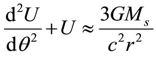
Suppose that a ray with the radian frequency  is coming from the surface of a star of radius
  and of mass
  to the surface of the earth which is x distance away from the centre of a star. As per our previous discussion, electromagnetic energy has the same acceleration as that of material bodies as well as point charges in the same gravitational field.
Let  be the gravitational acceleration of a ray on the surface of a star and
  be the gravitational aceleration of the same ray when it is on the surface of the earth.
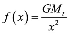
Then, we have from the law of gravitation [18],
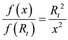 (101)
(101)
(Remembering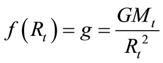 ),
),
 . (102)
Now, for the rectilinear motion of the ray towards OX direction, we have,
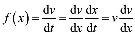 . (103)
Therefore, the differential equation for the velocity of the ray should read, from Equations (101-103),
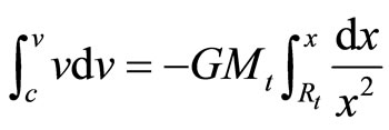 (104)
(104)
where c is the velocity of the ray on the surface of the star and v is the velocity of the same ray on the surface of the earth. From which we have,
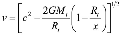 (105)
(105)
Therefore,
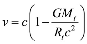 (106)
(106)
when x is large.
From which we have,
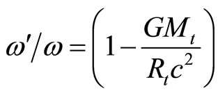 (107)
(107)
( is the radian frequency of the same light ray at the surface of the earth), as the number of complete waves passing through a point (i.e., frequency) must be proportional to the velocity of the waves .
4. Gravitation and Puzzling Electrodynamic Phenomena
Maxwell’s equations of electromagnetic fields are applicable only in free space and inside systems stationary in free space. One would then expect some corrections/modifications of Maxwell’s equations when the electromagnetic phenomena are studied on the surface of the earth which is moving with a high velocity in the free space. But those corrections are not needed!
All electrodynamic phenomena like reflection, refracttion, diffraction, interference etc., as observed on the surface of the earth, either with star light or with earth light are independent of the movement of this planet. That is: the earth’s surface is exactly equivalent to free space for our description of electromagnetic phenomena on it.
Just like electric charges and electromagnetic energy, electromagnetic fields possess momentum and energy which we could experience with our sense organs. Therefore, electromagnetic fields, too, are real physical entities (objects). All physical objects at the surroundings of the earth are carried with the earth. Therefore, the electric and magnetic fields existing at the near vicinity of the earth’s surface, should spin, translate, and rotate with the earth.
4.1. The Michelson-Morley Type Experiments in Air and Water
This will at once explain the null results of all the Michelson-Morley type Experiments in air and the Mascart-Jamin type Experiment in water at rest on the earth’s surface; and may give us some insight to understand why all electromagnetic phenomena as observed on the surface of the earth are independent of the motion of this planet [19].
4.2. The Kennedy-Thorndike Experiment
Electromagnetic radiation is the propagation of vibration of electric and magnetic fields. In the Kennedy-Thorndike experiment, it is observed that the velocity of light on the surface of the earth is independent of spinning of the earth around its axis [contra vide (4.7.)].
4.3. The Tomaschek (1924) and Miller’s Experiment (1925)
Where the Michelson-Morley experiment has been performed with starlight and sunlight, similar null results have been confirmed.
This can only happen if the electric and magnetic fields originating either from the earth, stars or from the Sun and existing at the near vicinity of the earth’s surface, spin, translate and rotate with the earth.
4.4. The Trouton-Noble Experiment (1904)
In a laboratory, when a charged condenser moves, the electric field around it changes and thereby a magnetic field is created. If the electric field originating from the condenser would move along with the condenser, there would be no change of electric field around the condenser and thereby, there would be no magnetic field around it.
Now, a condenser at rest on the earth’s surface moves with the earth. But the electric field around the condenser, too, moves with it. And therefore, the Trouton-Noble Experiment (1904) fails to detect any magnetic field around the condenser. This implies that the earth carries the condenser along with its electric field.
4.5. Sagnac Experiment
As per classical electrodynamics, light signals, divided in two parts and sent in opposite directions around a fixed circuit on a spinning disk, should not return to the point of division at the same instant. Because, the speed of light on a spinning disk is c – w when the light beam travels towards the direction of spinning of the disk, and c + w when the light beam travels in the opposite direction, w being the spinning velocity of the point on the disk where the speed of light is being measured. This effect is the primary effect of spinning. The actual experiment confirms this. This effect of light on a spinning disk was observed by G. Sagnac in an interferometer fixed on the disk in 1913 and is known as the Sagnac effect. But the earth’s motion seems to have no effect on the result. The implication is the same as stated in the previous examples.
4.6. The Observations of Bradley (1728), Airy (1871) and Zapffe (1992) on Aberration of Light
Aberration of Astral and Terrestrial Light
1) Suppose a ray from an overhead fixed star is coming to the earth which is moving with respect to the fixed star with a velocity u normal to the ray.
From the consideration of the relative velocity of classical physics, the man on the earth should see the star not on overhead through a telescope. Instead he should see the star deflected at an angle  towards the direction of motion of the earth from overhead such that
 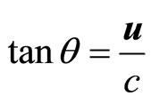 where c is the velocity of the ray in space fixed with the fixed star. Now if the telescope be filled with water, the man should see the star at an angle
  (such that
 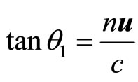 ) deflected towards the direction of motion of the earth from overhead, n being the refractive index of water.
In this case, the ray velocity and the phase velocity of the wave coming from the star will be different. The direction of the ray is here is the apparent direction and a ray coming from a mountain top should have the same aberration as given in the above analysis. For, the ray as per Maxwell should propagate with a velocity c with respect to free space which could be conceived as fixed with the fixed stars.
2) Now if the stars and the planets carry electric and magnetic fields along with them at their surroundings, a ray from an overhead fixed star will reach the surrounding of the sun and the ray will be carried with the sun. Then it will proceed and strike the electric and magnetic fields at the near vicinity of earth’s surface at an angle  deflected towards the direction of the motion of the earth from overhead such that
 , in case the earth is moving with respect to the sun with a velocity u normal to the ray and c is the velocity of light in the solar space; and the ray will be carried with the earth. The ray and its direction here are real.
On the surface of the earth, in this case, there is no relative motion between the ray and the earth towards the direction of motion of the earth. Therefore, a man on earth will see the star with an angle  tilted towards the direction of motion of the earth from overhead (as was observed by Bradley). If he fills the telescope with water, the ray velocity inside water must be c/n. But as there is no relative velocity between the ray inside water and the earth towards the direction of motion of the earth, the position of the star will not alter (i.e, there will be no further aberration as observed by Airy). Here the ray velocity and the phase velocity are the same and the ray and its direction in both the instances are real.
More interestingly, in such a situation, a ray coming from a mountain top should have no aberration as per Zapffe’s (1992) report [20].
All experiments conform to the case 2).
Therefore, we may conclude that electromagnetic fields are real physical entities, and that, as the earth spins about its axis, translates and rotates in its orbit, electric fields and magnetic fields originating either from the earth, stars or from the sun and existing at the near vicinity of the earth’s surface, spin, translate and rotate with the earth, exactly in the same way as other physical objects on the earth do.
This indicates that the velocity of light is subject to the influence of the gravitational field of the earth and this has been confirmed by many experiments. Therefore, it is likely that the centrifugal force and especially the Coriolis force originating from the spinning of the earth should also act on the propagation of light which have not been taken into consideration for the explanation of the results of the Michelson-Gale type experiments as proposed by Michelson-Gale, Kelly, Marmet and others.
4.7. The Experiments of Michelson-Gale and Bilger et al.
The earth just like all other physical objects carries light with it at the vicinity of its surface. Therefore, Coriolis force due to the rotation of the earth must act on the direction of propagation of light on the surface of the earth. This will explain the Michelson-Gale experiment and the experiment of Bilger et al. [21].
Let us choose a point O on the surface of the earth with the latitude  North and construct a tangential plane at this point. Now let us fix a Cartesian co-ordinate system in the plane such that OY represents the North and OX represents the East. Now suppose that the earth is not rotating and an element of light beam is arranged to move from a point P in the OY axis at the instant
  in a small circular motion in the clockwise direction such that at the time
  it touches the point Q in the OX axis and say
 . That is when
  and when
 .
.
Now suppose that the earth rotates with an angular velocity . Then the Coriolis force due to the rotation of the earth should deflect the beam mainly eastwardly and the beam will not touch the point Q. Instead it will touch a point R very adjacent to the OX axis. Now for a rough calculation of the distance OR, let us consider the motion of the beam on the OY axis with a velocity c from the point P to the point O. In this case, we may write,
 (108)
(108)
 (109)
(109)
 (110)
(110)
 (111)
(111)
Remembering the initial condition and taking into account
 (112)
(112)
We have,
 (113)
(113)
which is the deflection of the beam towards OX axis for a small circle. Therefore, in that case we have,
 (114)
(114)
For the beam moving in the anticlockwise direction, this distance will be
 (115)
(115)
From the last two equations we have for one complete rotation
 (116)
(116)
where A is the area of the circle. Fringe shifts relating to Equation (116) seem to be verified by the Experiments of Michelson-Gale and Bilger et al. [21]. The result will remain more or less the same when the circle is large.
(Stokes assumes that ether near the earth’s surface translates with the earth, but it does not rotate along with the rotation of this planet which could explain the experiments of Michelson-Gale and Bilger et al. In that case the magnetic field due to a system of charges slowly moving at a point on the earth’s equator with a velocity u with respect to the earth’s surface eastward would be almost double the magnetic field of the same system of charges moving similarly at 60˚ latitude when w  u, w being the rotational velocity of that point of the earth with respect to ether. This is impossible and so the assumption of Stokes too).
5. Conclusions
The deduction of the E-field and the B-field of a steadily moving point charge by Heaviside is a pioneering work in the nineteenth century. Depending on this deduction, we have deduced the electromagnetic momentum, the longitudinal and transverse electromagnetic masses of a steadily moving point charge classically. With the use of these results, we have explained classically the phenomena of increment of life spans of steadily moving radioactive particles, Thomas Precession, Transverse Doppler Effect and the fringe shift measured in the Fizeau Experiment.
We know from classical physics that electric charges, electric & magnetic fields and electromagnetic energy possess momentum and energy which we could experience with our sense organs. Therefore, all these are real physical entities (objects). All physical objects are subject to gravitation. Therefore, electromagnetic entities should similarly be subject to gravitation. This consideration immediately explains advance of perihelion of Mercury, bending of light rays grazing the surface of the sun and gravitational red shift.
Now, all physical objects at the surrounding of the earth are carried with the earth. Electromagnetic fields should similarly be carried with the earth. This at once explains the null result of the Michelson-Morley type experiments with terrestrial, solar and astral light, Sagnac Effect on a rotating disk on earth, stellar aberrations as observed by Bradley through a telescope filled with air, no further aberration as observed by Airy through a telescope filled with water and no aberration from a mountain top as reported by Zapffe (1992) [20]. The Coriolis force (originating from the spinning earth) that acts on the light beam explains the Michelson-Gale experiment and the experiments of Bilger et al. [21].
All those explanations demonstrate the non necessity of the invariant proposition as well as the space-time curvature propositions of Einstein.
The analysis shows that the superiority of the theory of relativity—special & general—over classical physics as advocated and publicized by the mainstream physicists is myth.
6. Acknowledgements
To write this article I have been encouraged with the writings of Late Debabrata Ghosh [22] of Reserve Bank of India, Kolkata-1, Late Prof. K. C. Kar [23], founder of the Indian Institute of Theoretical Physics, Calcutta and Dr. M. C. Duffy, Editor of the Proceedings of PIRT Conferences, 1988-, London. I thank T. K. Basu, and Somdeb Seal for their kind help to prepare the manuscript.
REFERENCES
- O. Heaviside, “The Electromagnetic Effect of Moving Point Charge,” The Electrician, Vol. 22, 1888, pp. 147- 148.
- O. Heaviside, “On the Electromagnetic Effects Due to the Motion of Electricity through a Dielectric,” Philosophical Magazine, Vol. 27, No. 5, 1889, pp. 324-339.
- J. J. Thomson, “On the Magnetic Effects Produced by Motion in the Electric Field,” Philosophical Magazine, Vol. 28, No. 170, 1889, pp. 1-14.
- H. A. Lorentz, “The Theory of Electron,” Dover Publications Inc., New York, 1951, pp. 35-36, 245-246.
- S. Hajra, “The Cross Radial Force,” Proceedings, Natural Philosophy Alliance, Vol. 8, College Park, 2011, pp. 235- 240.
- W. B. Morton, “Notes on the Electromagnetic Theory of Moving Charges,” Philosophical Magazine, Vol. 41, 1896, pp. 488-494.
- E. T. Whittaker, “A History of the Theories of Aether and Electricity,” Longmans, Green, and Co., London, 1910, pp. 341-342.
- J. R. Oppenheimer, “Lecture on Electrodynamics,” Gordon and Breach Science Publishers, New York, 1970, pp. 57-58.
- A. L. Miller, “Albert Einstein’s Special Theory of Relativity,” Springer, Berlin, 1981, pp. 98-99.
- A. Liénard, “Champ Électrique et Magnétique,” L’Éclairage Électrique, Vol. 16, No. 27-29, 1898, pp. 5-14, 53-59, 106- 112.
- E. Wiechert, “Elektrodynamische Elementargesetze,” Archives Néerlandaises, Vol. 5, 1900, pp. 549-573.
- O. D. Jefimenko, “Direct Calculation of the Electric and Magnetic Fields of an Electric Point Charge Moving with Constant Velocity,” American Journal of Physics, Vol. 62, No. 1, 1994, pp. 79-85. doi:10.1119/1.17716
- O. Heaviside, “Electric Papers, Vol. 2,” Macmillan and Company, New York and London, 1892, p. 514.
- S. Hajra, “Collapse of GRT: EM Interaction with Gravity derived from Maxwell and Newton,” Galilean Electrodynamics, Vol. 18, No. 4, 2007, pp. 73-76.
- S. Hajra, “A Study on the Interaction of Gravitating Fields with Electromagnetic Entities,” Journal of Gravitational Physics, Vol. 2, No. 2, 2008, pp. 7-22.
- R. P. Feynman, R. B. Leighton and M. Sands, “The Feynman Lectures on Physics, Vol. 1,” Narosa Publishing House, New Delhi, 1998, p. 23.
- R. P. Feynman, R. B. Leighton and M. Sands, “The Feynman Lectures on Physics, Vol. 3,” Narosa Publishing House, New Delhi, 1998, p. 1405.
- V. M. Starzhinskii, “An Advance Course of Theoretical Mechanics,” Mir Publishers, Moscow, 1982, pp. 264-265.
- S. Hajra, “A Critical Analysis of Special Relativity,” Proceedings, Physical Interpretations of Relativity Theory, London, 2000, p. 146.
- C. A. Zapffe, “Bradley Aberration and Einstein Space Time,” Indian Journal of Theoretical Physics, Vol. 40, 1992, pp. 145-148.
- H. R. Bilger, G. E. Stedman, Z. Li, U. Schreiber and M. Schneider, “Ring Lasers for Geodesy,” IEEE Transactions on Instrumentation and Measurement, Vol. 44, No. 2, 1995, pp. 469-470. doi:10.1109/19.377882
- D. Ghosh, “The Michelson-Morley Experiment,” Indian Journal of Theoretical Physics, Vol. 42, No. 3, 1994, pp. 73-79.
- K. C. Kar, “A New Approach to the Theory of Relativity,” Institute of Theoretical Physics, Calcutta, 1970, pp. 52-57.