Journal of Modern Physics
Vol. 2 No. 8 (2011) , Article ID: 6678 , 7 pages DOI:10.4236/jmp.2011.28098
The Cosmological Evolution of Baryonic Matter’s Density Perturbations under Influence of the Quintessence
V. G. Fessenkov Astrophysical Institute, National Centre for Cosmic Researches and Technologies, National Space Agency, Almaty, Kazakhstan
E-mail: chechin@aphi.kz
Received March 28, 2011; revised May 15, 2011; accepted June 6, 2011
Keywords: Baryonic Matter’s Density Perturbations, Quintessence Field, Nonstationary Equation of State of the Universe
ABSTRACT
For deeper understanding the process of baryonic matter evolution in the expanding Universe it is necessary to know the physical property of concrete field that represents the background of substrate type of dark energy. Beside, it is necessary to explore in details the influence of such field on the continuous medium of baryonic matter. These statements were realized for the quintessence field that describes by two gravitating scalar fields. They give own contributions at the total pressure and at the total mass density of baryonic matter. It allowed show that evolution of baryonic matter’s density perturbations obeys the equation of forced oscillations and admits the resonance case, when amplitude of baryonic matter’s density perturbations gets the strong short-time splash. This splash interprets as a new macroscopic mechanism of the initial matter density perturbations appearance.
1. Introduction
The evolution of baryonic matter from its density fluctuations appearance up to the processes of galaxies origin is one of the most important problems for modern cosmology [1,2]. This theme was considered as in Newtonian cosmology and as in the framework of relativistic cosmology from different sides (see, for example, [3,4]). Some current tendencies in this problem, in particular, are lighting in articles [5,6].
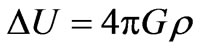
We’ll focus this paper on another aspect of this problem. Namely, in many articles the influence of different cosmological substrates on the evolution of baryonic matter’s perturbations was reduced to setting their equations of state, i.e. to setting parameter . As the result it leads to setting the different expressions of Hubble constant in the “friction term” of the basic equation
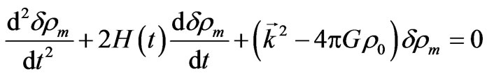 that describes the evolution of baryonic matter’s density perturbations. However, this approach allows consider such evolution as the process that elapses on the background of nonbaryonic cosmic substrate, only (and even stay in shadow the physical properties of this substrate).
But in realty this substrate interacts with baryonic matter in definite way. That is why it is essential to consider its influence on the baryonic matter evolution in details. Lower it will be shown that chosen variant of substance (quintessence field with parameter ) describes as small time-increasing field
  on the background of constant scalar field
 , while chosen variant of baryonic matter describes as small wave-type fluctuations
on the background of uniformly distributed motionless gas with nonvariable mass density . Thus we have the system of two small fields (
 and
and ) that evolves on the stable background of
  and
and .
.
Such problem wording, hence, is analogous to those in cosmology where the multi-fluids evolution searches [7-10] and, more generally, in hydrodynamics where the motion of poly-component media examines (see, for example, [11,12]). Beside, for the closed to our physical system (scalar field and perfect fluid) the properties of cosmological density perturbations were considered in article [13]. Mark, that opposite physical situation is permissible, also. In fact, the cosmological evolution of two coupled scalar fields in the presence of a barotropic fluid was examined in [14].
It is also necessary to enumerate some articles where different aspects of the mutual interaction between baryonic matter and quintessence were examined. In fact, in [15] was estimated the amplitude of perturbation in dark energy at different length scales for a quintessence model with an exponential potential; in [16-18] was considered the growth of perturbations in dark matter coupled with quintessence.
Some other cosmological aspects of quintessence existence were done in [19].
This article organized as follows. In Section 2, we demonstrate that two scalar fields can describe the physical properties of quintessence field. (Mark that variant of the quintessence description by two scalar fields, similar to our, have been proposed in [20]. Two-scalar fields approach for the dark energy description was considered in [21], also). Section 3 devotes to searching the evolution of scalar field  that represents as small standing waves on the background of basic scalar field
 . Section 4 is devoted to exploring the influence of field
  on the evolution of baryonic matter’s density perturbations. In Section 5 we examine the effect of stimulation the baryonic matter’s density perturbations growing by scalar field
 . Our conclusions are presented in Section 6, finally.
2. Scalar Fields Representing the Quintessence Field
One of the actual problems for modern cosmology is the theoretical description of quintessence field—one type of dark energy. Its observable properties are the scale homogeneity and the absence of clustering [22]. Quintessence is described by an ordinary scalar field minimally coupled to gravity, but with particular potentials that lead to late time inflation [23]. The action for quintessence is given by
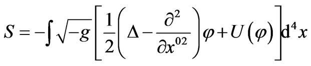 (1)
(1)
where  is the 3-dimensional Laplace operator,
 — potential of any scalar field.
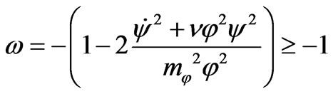
The simplest equation of state for any type of dark energy usually chooses in the linear form , where magnitude of
  lays within the interval
[24]. Therefore
 (2)
(2)
Later on we’ll describe arbitrary quintessential field  by coupled scalar fields—ordinary
  and Higgstype
 .
.
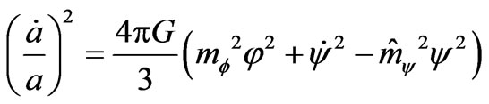
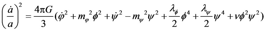
Thus consider the self-consistent problem for the mutual evolution of fields and Universe. The corresponding system of Einstein’s equations and equations of two interacting scalar fields is
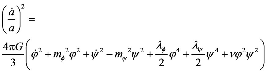 (3)
(3)
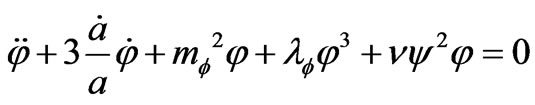 (4)
(4)
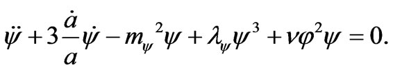 (5)
(5)
Let masses and fields correlate each other as 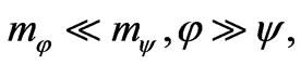 while the self-action coefficients fulfill inequality—
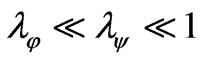 . Hence, the period of oscillations for field
  is essentially larger than the period of oscillations for field
  (
(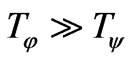 ) and
) and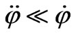 , accordingly. In another words, in time of field
  changing the basic field
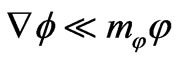
  don’t change practically, i.e. we may describe it by the conditions
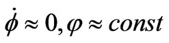 (6)
(6)
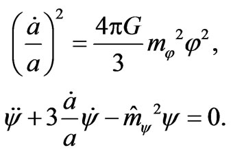
After neglecting the fields’ self-actions we get the simplified system of equations
 (7)
(7)
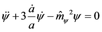 (8)
(8)
which will be under our analyzes. Here 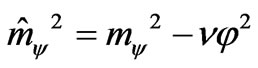 is the squared field’s
  effective mass that determines by field mass
  and its interaction with field
 .
.
Later on it is necessary to set masses of scalar fields and their initial amplitudes. According [25] their typical magnitudes are
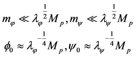 (9)
(9)
where  is the Planckian mass. Having in mind these constrains, consider the case when
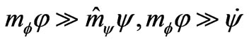 (10)
(10)
Moreover, for our model the inequalities (15) take place if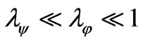 . Conditions (10) indicate that energy of basic field
  is essentially larger than energy of additional field
 . Under this assumption the system (9)-(10) takes on more simple form
 (11)
(11)
Equation (11) reduce to one linear differential equation of the second order 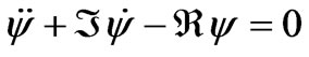 with coefficients
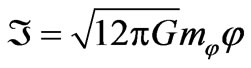 ,
, . Its solutions we’ll look for in the standard exponential form
 . Hence, we get the algebraic equation
  that has two roots:
 (12)
(12)
From (9) and (10) it follows that . This condition allows to decompose the expression under root sign into the Taylor series with respect to small value
 , and to get two solutions
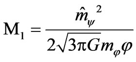 ,
,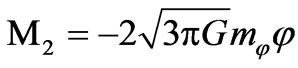 (13)
(13)
Note also, that second of them is the approximate solution of zeroth accuracy with respect to the ratio . Thus the sought-for solutions of field
  we may take in the forms
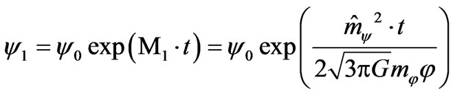 (14)
(14)
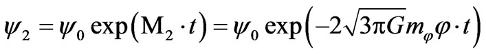 (15)
(15)
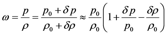
From (9)-(11) it is unproblematic to find the additives to energy density and to pressure
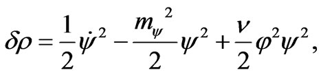 (16)
(16)
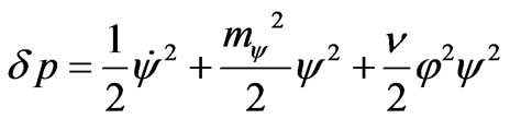 (17)
(17)
while the main items are
 ,
, (18)
(18)
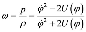
From (16)-(18) it is easy to verify that these two scalar fields describe the quintessence field. In fact, from (2) we get
 (19)
(19)
Due to condition (6) and (18) we see that ordinary scalar field  is in the vacuum state, i.e.,
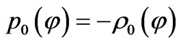 . Hence
 (20)
(20)
Therefore two coupled scalar fields describe the quintessential state of dark energy.
3. The Scalar Field  Evolution
Let the fields  and
and  possess any space inhomogeneity. (Another type of the inhomogeneous quintessence model has been proposed in [26].) Under the conditions
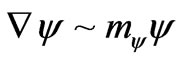 ,
,  this leads to the system
 (21)
(21)
 (22)
(22)
 (23)
(23)
Here we take into account that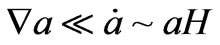 , also.
For solving this system put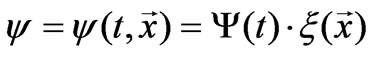 , where
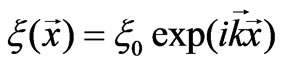 . Last expression indicates that perturbed potential is the plane wave with the timevariable amplitude,
  its wave vector. Such choice is analogous to Jeans’ presentation of the perturbations in baryonic substrate.
Substitution all of them into Equation (23) will arrive it to the following one
 (24)
(24)
with the nonzero right part. It is easy to see that
 . Hence the following equation leads from (24) one
 (25)
(25)
With the needed accuracy (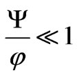 ) we have
and 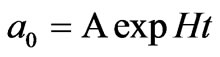 with arbitrary amplitude
 . After neglecting the field self-interaction we get equation
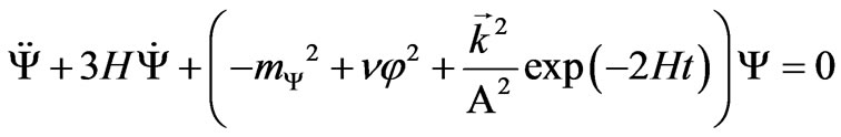 (26)
(26)
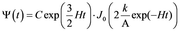
whose exact partial solution, in accordance [27], expresses as
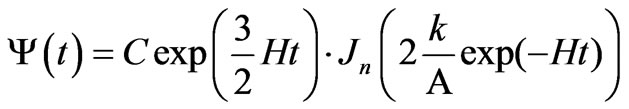 (27)
(27)
where
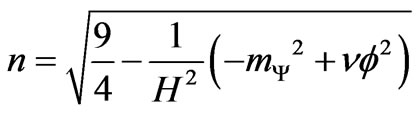
is the index of Bessel function,  is an arbitrary constant.
Let 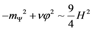
for simplicity, then  and
and
 . Furthermoreassuming that
 , the field potential takes on the form
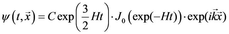 (28)
(28)
Now examine the behavior of this function in time. Let  is the dimensionless time. Using the numerical and the graphical representations of Bessel functions [28] we see that at large argument (
 ) function
 . However, for our purpose we must consider the opposite situation when
 .
.
For doing this consider the series representation of Bessel function of zeroth order
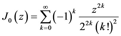 (29)
(29)
and limit ourselves by first two terms only, because it rapidly (~ ) decreases with
  growing. Hence,
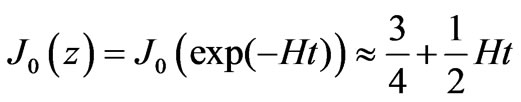
and function (28) reduces to the next one
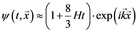 (30)
(30)
if . This important result—time-increasing amplitude—allows lighting the process of baryonic matter’s macroscopic perturbations growth from new side.
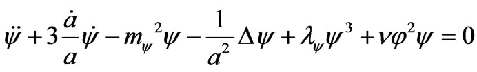
4. Influence of Field  on the Baryonic Matter’s Density Perturbations Growing
Our next step is searching the influence of field  on the baryonic matter’s density perturbations growing. Later on we’ll base on the Jeans equations for adiabatic case.
In the usual designations (together with the equation of state for baryonic matter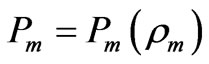 ) they are
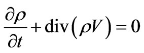 (31)
(31)
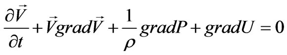 (32)
(32)
 . (33)
For enriching our goal it is necessary to use the wellknown method of description the poly-components fluid dynamics. Namely, for searching the microscopic perturbations of baryonic matter specify them in the standard manner [29,30]
 (34)
(34)
 , (35)
 (36)
(36)
 (37)
(37)
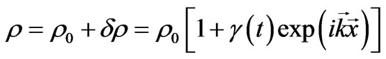
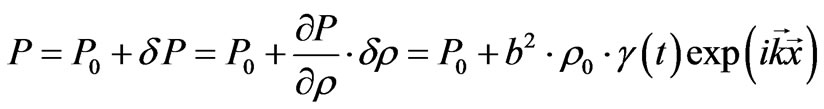
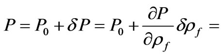
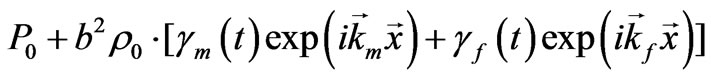
Beside, as we consider the influence of baryonic matter on the background of phantom field, it is needed to take into account that last will contribute its additions at the pressure  and at the mass density
 . Hence,
  , and
, and . Moreover, according our assumption we have
 ,
, (38)
(38)
 ,
, (39)
(39)
where ,
,  ,
,  and
and  are the small perturbed additions to initials mass densities
 ,
,  and to initial pressures
 ,
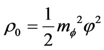
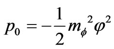
, . In our case, the main terms for mass density and for pressure, that associated with vacuum and determined by the field
 , are
, are
 ,
, 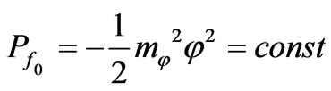 (40)
(40)
while the corresponding additions have the forms (we neglect the fields interaction, for simplicity)
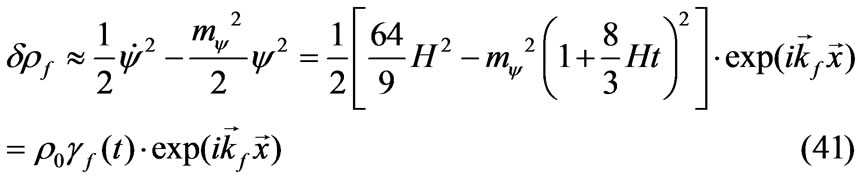
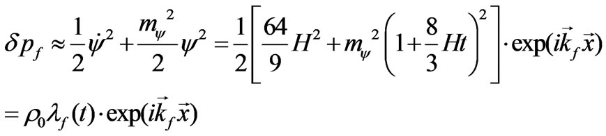 (42)
(42)
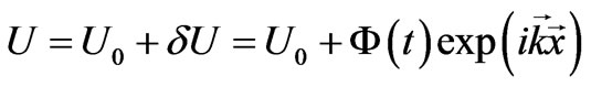
That is why the variables in (34)-(37) may be represent as
 (43)
(43)
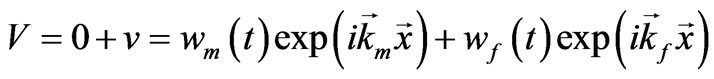 (44)
(44)
 (45)
(45)
 (46)
(46)
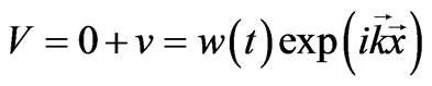
where we assume that speeds of sound in a baryonic matter and in the quintessence field are equal each other, i.e., . Beside, for next simplification let
  (in [31] it was considered the bi-velocities type of fluid with special nonzero components) and for the case of dust-like baryonic substance imply that
 . Whence it results
 ,
, .
.
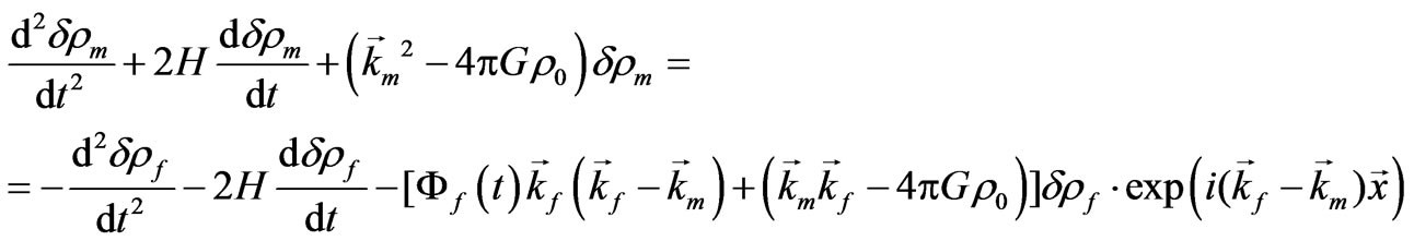
Substituting (43)-(45) into (31)-(33) and making required transformations, we get the dynamical equation of two-component media.
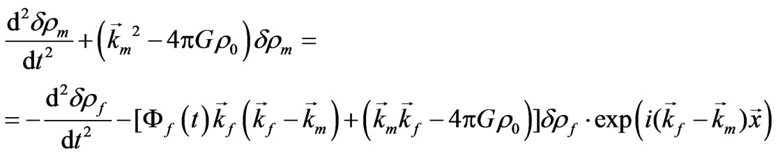 (47)
(47)
where 
Later on, assuming that  and accounting (46) the previous equation goes into
 (48)
(48)
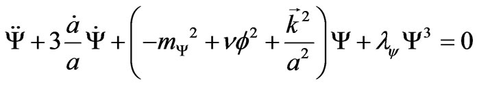
The most attractive consequence of this equation, that has the evolutionary nature, we get after the omitting constant values in third term and replacing
 by
by 
(due to minuteness  here and after). Thus the standard equation of forced oscillations
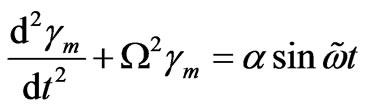 (49)
(49)
takes place, where
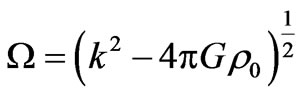
is the basic internal frequency,
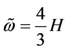 and
and 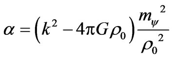 are the externals frequency and amplitude, accordingly.
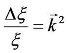
Now it should be pointed out that condition
relates to the resonance case. Hence, the amplitude of baryonic matter’s density perturbations gets the strong short-time splash. This result is very significant, because the splash may be real macroscopic mechanism of an initial matter density perturbations appearance. Moreover, the above mention condition determines the resonancecase wave vector
 .
.
In other—nonresonance—cases ( ) the amplitude of oscillations, according standard theory [32], at times
  (see Section 3) becomes growth linearly, i.e.
 . So, it stimulates the process of matter’s density perturbations increasing (see next Section 5).
5. Effect of Stimulation the Baryonic Matter Density Perturbations Growing
Point out that according to above considered behavior of field  (Equations (13) or (39)) it is necessary to generalize Equation (47) in the similar manner. The result is obvious
 (50)
(50)
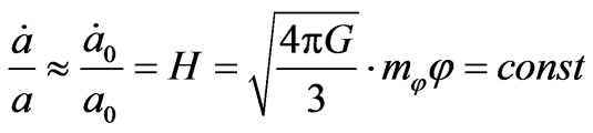
where the Hubble constant is
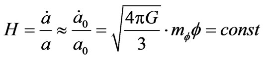 .
.
The “friction term” in right side of (50) will alter the amplitude and frequency of forced oscillations in (49) owing to previous results, but don’t change the key conclusion of Section 4—the linear time-growing of baryonic matter’s perturbations. As for the “friction term” in left side of (50) it is necessary to say follow.
The problem of baryonic matter perturbations growing in the dust-like Universe with nonvariable Hubble constant was considered in number of recent articles (see, for example [33-38]). But their common result adequate to those in [29,30]—the amplitude of perturbations increases as different powers of time, i.e., 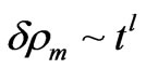 , where, in particular,
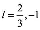 etc. More complicate results take place when Hubble constant is the time-varying value [39]. For instance, in article [40] it was shown that then
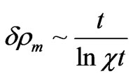 .
.
Summarize, in all of these cases the “friction term”
at Jeans-like equation leads to main consequence—the growing of baryonic matter perturbations in the expanding Universe.
Hence, for baryonic Universe the matter density perturbation will develop in time more rapidly, namely as
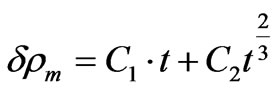 (51)
(51)
where  and
and  are any suitable constants.
That is why our result describes the effect of stimulation the baryonic matter’s density perturbations growing by quintessence field.
6. Conclusions
Here it was shown that for deeper searching the process of baryonic matter evolution in the expanding Universe it is necessary to:
1) know the physical property of concrete field (or fields) that represents the background of nonbaryonic substrate type of dark energy, and 2) take into account the influence of such field on the continuous medium of baryonic matter.
In our article these statements were realized for the quintessential field. As the result we describe quintessence by two gravitating scalar fields. First of them is the invariable field , while the second evolves as the space-wave with linearly growing amplitude (30). These fields give their contributions at the total pressure
  and at the total mass density
  of baryonic matter. As a consequence the evolution of baryonic matter density perturbations obeys the standard equation of forced oscillations (49) and admits the resonance case, when amplitude of baryonic matter density perturbations gets the strong short-time splash. This splash was interpreted as the macroscopic mechanism of initial matter’s density perturbations appearance.
In other—nonresonance—cases the amplitude of oscillations becomes growth linearly in time. That is why it also may stimulate the process of matter density perturbations increasing accord the expression (51).
As a result it is possible to say that quintessence field highly actively affects on the baryonic matter’s density perturbation growing in the Universe.
REFERENCES
- V. L. Ginzburg, “On Some Advances in Physics and Astronomy over the Past Three Years,” Physics–Uspekhi (Advances in Physics Sciences), Vol. 45, No. 2, 2002, pp. 205-211.
- A. Sandage, “The Universe at Large,” In: G. Munch, A. Mampaso and F. Sanchez, Eds., Cambridge University Press, Cambridge, 1997.
- Ya. B. Zel’dovich and I. D. Novikov, “Relativistic Astrophysics,” Vol. 2, Chicago Press, Chicago, 1983.
- T. Padmanabhan, “Structure Formation in the Universe,” Cambridge University Press, Cambridge, 1993.
- G. Dvali, A. Gruzinov and M. Zaldarriaga, “Cosmological Perturbations from Reheating, Freezeout, and Mass Domination,” Physical Review D, Vol. 69, 2003, 023505, [arXiv:astro-ph/00306052].
- D. Polarsky and R. Gannouji, “On the Growth of Linear Perturbations,” Physics Letters, Vol. B660, 2008, p. 439; arXiv: 0710.1510v2 [astro-ph] 11 October 2007, pp. 1-8.
- F. Verheest, P. K. Shukla, G. Jacobs and V. V. Yaroshenko, “Jeans Instability in Partially Ionized SelfGravitating Dusty Plasmas”, Physical Review E, Vol. 68, 2003, pp. 1-4.
- M. C. Johnson and M. Kamionkowski, “Dynamical and Gravitational Instability of Oscillating-Field Dark Energy and Dark Matter,” Physical Review D, Vol. 78, 2008, pp. 1-9.
- T. A. Thompson, “Gravitational Instability in Radiation Pressure-Dominated Backgrounds,” Astrophysical Journal, Vol. 684, No. 1, 2008, pp. 212- 225.
- P. K. S. Dunsby, “Gauge-Invariant Perturbations in Multi-Component Fluid Cosmologies,” Classical and Quantum Gravity, Vol. 8, 1991, pp. 1785-1806. doi:10.1088/0264-9381/8/10/006
- L. T. Chyornyj, “The Relativistic Models of Continuous Media,” Nauka, Moscow, 1983, (in Russian);
- S. A. Serov and S. S. Serova, “Multi-Component Gas-Dynamics and Turbulence,” 2005, E-print, arXiv: physics/0503215.
- N. Bartolo, P.-S. Corasaniti, A. Liddle and M. Malquarti, “Perturbations in Cosmologies with a Scalar Field and a Perfect Fluid,” Physical Review D, Vol. 70, 2004, 043532, arXiv: astro-ph/0311503v3, 22 April, 2004, pp. 1-9.
- A. De la Macorra, “Interacting Dark Energy: Generic Cosmological Evolution for Two Scalar Fields,” Journal of Cosmology and Astroparticle Physics, Vol. 1, 2008, p. 30. doi:10.1088/1475-7516/2008/01/030
- S. Unnikrishnan, H. K. Jassal and T. R. Seshadri, “Scalar Field Dark Energy Perturbations and Their Scale Dependence,” Vol. 78, No. 12, 2008, pp. 1-12. arXiv: astro-ph 0801.2017v3,
- T. Koivisto, “Growth of Perturbations in Dark Matter Coupled with Quintessence,” 2005, pp. 1-14, arXiv: astro-ph/0504571v2.
- V. Sahni and W. Limin, “A New Cosmological Model of Quintessence and Dark Matter,” Physical Review, Vol. D62, 1999, pp. 1-4, arXiv:astro-ph/9910097v3.
- P. J. E. Peebles and A. Vilenkin, “Noninteracting Dark Matter,” 1998, pp. 1-9. arXiv:astro-ph/981059v1
- J. S. Alcaniz and J. A. S. Lima, “Dark Energy and the Epoch of Galaxy Formation,” The Astrophysical Journal, Vol. 550, No. 1, 2001, pp. L133-L136. doi:10.1086/319642
- M. C. Bento, O. Bertolami and N. C. Santos, “A TwoField Quintessence Model,” Physical Review D, Vol. 65, No. 6, 2002, pp. 1-4. arXiv:astro-ph/0106405v2
- X.-F. Zhang, H. Li, Y.-S. Piao and X. M. Zhang, “TwoField Models of Dark Energy with Equation of State Across-1,” Modern Physics Letters A, Vol. 21, 2005, pp. 1-5. arXiv:astro-ph/050152v1
- D. I. Podol’sky, “On the Equation of State for the Λ Field,” Astronomy Letters, Vol. 28, No. 7, 2002, pp. 434- 437.
- E. J. Copeland, M. Sami and Sh. Tsujikawa, “Dynamics of Dark Energy,” International Journal of Modern Physics D, Vol. 15, No. 11, pp. 1-94. arXiv: hep-th/0603057v3
- A. D. Chernin, “Cosmic Vacuum,” Physics-Uspekhi, (Advances in Physical Sciences), Vol. 44, No. 11, 2001, pp. 1099-1118.
- A. D. Linde, “Particle Physics and Inflationary Cosmology,” Harwood Academic Publishers, Chur, 1990.
- N. J. Nunes and D. F. Mota, “Structure Formation in Inhomogeneous Dark Energy Models,” Monthly Notices of the Royal Astronomical Society, Vol. 368, 2006, pp. 751- 758. arXiv:astro-ph/0409481v2
- E. Kamke, “Differentialgleichungen: Lösungsmethoden und Lösungen,” Leipzig, 1959.
- G. A. Watson, “Treatise on the Theory of Bessel Functions,” 2nd Edition, CUP, 1944.
- P. J. E. Peebles, “Physical Cosmology,” Princeton University, Princeton, 1971.
- S. Weinberg, “Gravitation and Cosmology,” John Wiley & Sons, Inc., New York, London, Sydney and Toronto, 1972.
- H. Brenner, “A Critical Test of Bivelocity Hydrodynamics for Mixtures,” Journal of Chemical Physics, Vol. 133, No. 15, 2010, pp. 154102-154102-8. doi:10.1063/1.3494028
- L. D. Landau and E. M. Lifshitz, “Mechanics,” Nauka, Moscow, 1958, (in Russian).
- A. D. Chernin, D. I. Nagirner and S. V. Starikova, “Growth Rate of Cosmological Perturbations in Standard Model: Explicit Analytical Solution,” Astronomy and Astrophysics, Vol. 399, No. 1, 2003, pp. 19-21.
- D. Munshi, C. Porciani and Yun Wang, “Galaxy Clustering and Dark Energy,” Monthly Notices of the Royal Astronomical Society, Vol. 349, No. 1, 2004, pp. 281-290.
- V. Linder and A. Jenkins, “The Cosmological Simulation Code GADGET-2,” Monthly Notices of the Royal Astronomical Society, Vol. 346, No. 2, 2003, pp. 573-583.
- W. J. Persival, “Cosmological Structure Formation in a Homogeneous Dark Energy Background,” Astronomy and Astrophysics, Vol. 443, No. 3, 2005, pp. 819-830.
- L. Wang and P. Steinhardt, “Cluster Abundance Constraints on Quintessence Models,” Astrophysical Journal, Vol. 508, 1998, pp. 483-490.
- N. J. Nunes, A. S. da Silva and N. Aghanim, “Number Counts in Homogeneous and Inhomogeneous Dark Energy Models,” Astronomy and Astrophysics, Vol. 450, No. 3, 2006, pp. 899-907. doi:10.1051/0004-6361:20053706
- S. Basilakos, “Cosmological Implications and Structure Formation from a Time Varying Vacuum,” Vol. 395, 2009, pp. 1-10. arXiv:0903.0452v1 [astro-ph. CO]
- L. M. Chechin, “Antigravitational Instability of Cosmic Substrate in Newtonian Cosmology,” Chinese Physics Letters, Vol. 23, No. 8, 2006, pp. 2344-2347. doi:10.1088/0256-307X/23/8/104