Applied Mathematics
Vol.07 No.18(2016), Article ID:73034,17 pages
10.4236/am.2016.718188
The Convergences Comparison between the Halley’s Method and Its Extended One Based on Formulas Derivation and Numerical Calculations
Shunji Horiguchi
Department of Economics, Niigata Sangyo University, Niigata, Japan

Copyright © 2016 by author and Scientific Research Publishing Inc.
This work is licensed under the Creative Commons Attribution International License (CC BY 4.0).
http://creativecommons.org/licenses/by/4.0/


Received: October 22, 2016; Accepted: December 24, 2016; Published: December 27, 2016
ABSTRACT
The purpose of this paper is that we give an extension of Halley’s method (Section 2), and the formulas to compare the convergences of the Halley’s method and extended one (Section 3). For extension of Halley’s method we give definition of function by variable transformation in Section 1. In Section 4 we do the numerical calculations of Halley’s method and extended one for elementary functions, compare these convergences, and confirm the theory. Under certain conditions we can confirm that the extended Halley’s method has better convergence or better approximation than Halley’s method.
Keywords:
Recurrence Formula, Newton’s Method, Halley’s Method, Extension of Halley’s Method, Third-Order Convergence

1. Introduction
In 1673, Yoshimasu Murase [1] made a cubic equation to obtain the thickness of a hearth. He introduced two kinds of recurrence formulas of square  and the deformation. We find that the three formulas lead to a Horner’s method (Horiguchi, [2] ) and an extension of Newton’s method (Horiguchi, [3] ). This shows originality of Wasan (mathematics developed in Japan) in the Edo era (1603-1868). We do research similar to Horiguchi, [3] against the Halley’s method. We give function
  defined from
  for extension of Halley’s method.
From now on, let  be a real number, and a function
  times differentiable if necessary, and
  continuous.
Definition 1.1. Let  where
where  is a real number that is not 0. We define the function g(t) such as
 (1)
(1)
Because , the graph of
  extends or contracts by
  in the
  -axis, without changing the height of
 . Expansion and contraction come to object in
  and
and .
.
Theorem 1.2. The formulas
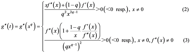
give the convex upward (the convex downward resp.) at the point  of graph of
 .
.
Proof. It is proved by the next calculations.
 (4)
(4)
 (5)
(5)
□
From the formulas (4), (5), we obtain the next theorem.
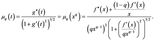
Theorem 1.3. The curvature of the cure  at the point
  is formulas (6) and (7).

These become the curvature  of
of  if
if  in particular.
Proof. Formula (6) is obtained by substituting the formulas (4) and (5) for  in the curvature
 . □
. □
Theorem 1.4. A necessary and sufficient condition for
 (8)
(8)
is that formula (9) holds.
 (9)
(9)
Proof. Formula (9) is obtained from (8). □
Proposition 1.5. If  is a simple root (
 multiple root resp.) of
 , then
  becomes the simple root (
 multiple root resp.) of
 .
.
2. Halley’s Method and Extension of Halley’s Method
Definition 2.1. The recurrence formula to approximate a root of the equation 
 (10)
(10)
is called Halley’s method1.
Halley’s method is obtained by improving the Newton’s method (11) (Ref. [5] ).
 (11)
(11)
They are methods of giving the initial value , calculating
  one after another, and to determine for a root.
From now on we omit the notation  in recurrence formulas. Applying the Halley’s method to
 , we get
 (12)
(12)
If we express this by formula (1) in , then we get the next definition.
Definition 2.2. Let α be a root of the equation . (13) is the recurrence formula to approximate
 . We call this the
  -th power of the extension of Halley’s method (EH-method).
 (13)
(13)
Here, if  then the formula (13) becomes Halley’s method.
Calculation formula of  -th power of EH-method is this.
 (14)
(14)
3. Formulas to Compare the Convergences for Extensions of Halley’s Method
Theorem 3.1. Let  be a simple root for
 , i.e.,
 . Then Halley’s method becomes the following third-order convergence.
 (15)
(15)
If  is
is  (
( ) multiple root, then it becomes the following linearly convergence.
 (16)
(16)
Proof. There is a brief proof of (15) in wikipedia [4] . Therefore we go to the proof of (16).
We merely sketch  with
with . Since
  is represented as
 (17)
(17)
 is as follows, respectively.
 (18)
(18)
From these formulas, we obtain the following linearly convergence.
 (19)
(19)

Lemma 3.2. In the sequence , let
, let , and
, and ,
,  an arbitrary real constant number that is not 0, respectively. In this case following formula holds for large enough integer
 .
.
 (20)
(20)
Proof. Applying L’Hospital’s rule to , formula (20) is obtained.
□
Theorem 3.3. Let the condition be the same as Theorem 3.1. If  sufficiently close to
 ,then
,then  -th power of EH-method (Extended Halley’s method) becomes the third-order convergence of the following formula.
 (21)
(21)
If  is
is  (
( ) multiple root, then it will be linearly convergence of the following formula.
 (22)
(22)
Proof. If  is a simple root for
 , then
  also becomes a simple root for
 . In this case Halley’s method for
  becomes the third-order convergence of the following formula.
 (23)
(23)
Here  become the followings.
 (24)
(24)
Therefore we obtain
 (25)
(25)
By lemma 3.2, we get
 (26)
(26)
Therefore, formula (25) becomes
 (27)
(27)
By changing the independent variable  of the functions
  and
and  in numerator to
 , we obtain (21).
In case that  is
is  multiple root, by (16), (1) and (20) we obtain
 (28)
(28)
□
Theorem 3.4. Let  be a simple root of
 . Then a necessary and sufficient condition for the convergence to
  of
of  -th power of EH-method is equal to or faster than Halley’s method is that
  satisfies the following conditions.
 (29)
(29)
That is
 (30)
(30)
Proof. Compare the coefficient of  of the third-order convergence of
  -th power of EH-method and that in the case of Halley’s method. Then the necessary and sufficient condition is equivalent to the next formula.
 (31)
(31)
The formula (29) is obtained from this. □
Corollary 3.5. (1) If  then (30) becomes
 (32)
(32)
(2) If  then (30) becomes
 (33)
(33)
We transform the equation  into
into . That is, two equations have the same root.
  -th power of EH-method for
  is
is
 (34)
(34)
and if  is a simple root, then it becomes the third-order convergence (35).
 (35)
(35)
We get the following by comparing the coefficient of  of formula (21) and (35).
Proposition 3.6. Let , and
, and  a simple root. Then a necessary and sufficient condition for the convergence to
  of
of  -th power of EH-method (Extended Halley’s method) (13) of
  to be equal to or faster than that
  -th power of EH-method (34) of
  is that the real numbers
  and
and  satisfy the following condition (36).
 (36)
(36)
Theorem 3.7. Let  be a simple root for
 , i.e.,
 . Inequality (29) is represented by the second derivative
 (37)
(37)
which distinguishes the convex-concave of the curve . It shows the next complicated inequalities (38), (39).
(i) 
 (38)
(38)
(ii) 
 (39)
(39)
Proof. We lead inequalities (38), (39) from (29). Let
 (40)
(40)
Then inequality (29) becomes
 (41)
(41)
 (42)
(42)
We transform the formula B.
 (43)
(43)
Therefore inequality (29) becomes (44).
 (44)
(44)
Furthermore, we transform the inequality.
 (45)
(45)
From (45), we get (38), (39) according to plus, minus number of  respectively. □
Theorem 3.8. Let the condition be the same as the above Theorem. Inequality (29) is represented by the curvature
 (46)
(46)
Those are the next complicated inequalities (47) and (48).
(i) 
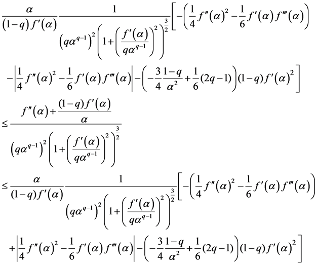 (47)
(47)
(ii) 
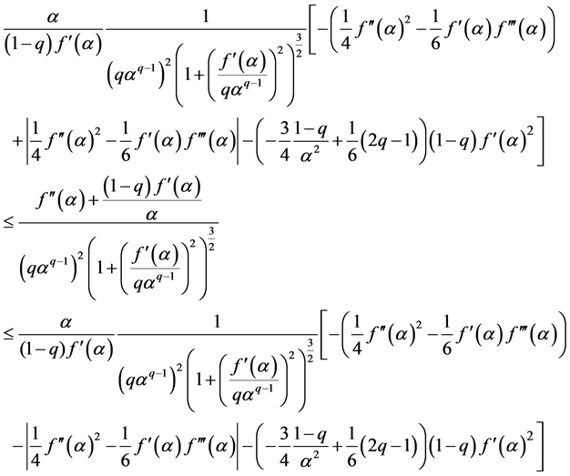 (48)
(48)
Proof. We get (47), (48) by dividing formula (38), (39) in , respectively.
4. Convergence Comparisons by the Numerical Calculations of Halley’s Method and Extensions of Halley’s Method
We perform numerical calculations by the calculation formula (14) in the standard format in Excel 2013 of Microsoft. We perform numerical calculations for various equations such as  -th order equations (
 ), equations of trigonometric, exponential, logarithmic function, respectively.
In the examples of the followings, there are cases where some numerical calculations do not fit in with the inequality (30) a little. Those are probably due to the formula (21) the approximate formula, choosing the initial value , and the accuracy of using the standard format in Excel is insufficient. However, the results to fit the theories generally have been obtained.
Example 4.1. A quadratic equation
 (49)
(49)
The roots of (49) are . Because
 , in case of
 , condition (33) becomes
 (50)
(50)
We choose real numbers  and initial values
  such as Table 1, Table 2, and do numerical computations. We explain how to read Table 1. The first column represents the initial value
  and the absolute error, and the first row represents the real number
  of
of .
.
Two numbers 1 and 1.11022E−16 of intersection of two row and two column mean the following.
Number 1 indicates the number of iterations that Halley’s method  to converge to the root 1. 1.11022E−16 indicates the absolute error |the value
  of the convergence of the numerical calculation―root 1|. If two iteration numbers are the same for the same initial value
 , then we evaluate the convergences by the absolute errors. In the Table 1, Table 2, all
  -th power of EH-method (Extension of Halley’s method) converge in root 1 at iteration number
 . But, for the same initial value
 , each column of EH-method
  has the absolute errors (at least one) that are equal to or smaller than Halley’s method
  in the ranges of (50).
We confirm Theorem 3.7. Because  in
in , inequality (39) is applied. In this case (39) becomes the following inequality.
 (51)
(51)
The results are Table 3. The range of  which satisfies (51) becomes
 .
.
Example 4.2. A cubic equation
 (52)
(52)
Because the root of (52) is 2, the condition (30) becomes
 (53)
(53)
We choose real numbers  and initial values
  such as Table 4, Table 5, and do numerical computations. All iteration numbers are 2 or 3. But, for the same initial value

Table 1. Calculations of (14) for root 1, −0.041 ≤ q ≤ 1.
Table 2. Calculations of (14) for root 1, 23 ≤ q ≤ 24.042.
Table 3. Calculations of (51) for root 1, −0.041 ≤ q ≤ 1.
Table 4. Calculations of (14) for root 2, −1.8875 ≤ q ≤ −1.462.
Table 5. Calculations of (14) for root 2, 1 ≤ q ≤ 1.4262.
 , each column of EH-method
  has the absolute errors (at least one) that are equal to or smaller than Halley’s method
  in the ranges of (53).
Example 4.3. A cubic equation
 (54)
(54)
In case of the root 1, the condition (30) becomes
 (55)
(55)
We choose real numbers  and initial values
  such as Table 6, Table 7, and do numerical computations. Each initial value
 , iteration number of EH-method
  and Halley’s method
  are the same. But, for the same initial value
 , each column of EH-method
  has the absolute errors (at least one) that are smaller than Halley’s method
  in the ranges of (55).
Example 4.4.
 (56)
(56)
The roots of (56) are  The condition (30) becomes
 (57)
(57)
If we take the root in , then (57) becomes
 (58)
(58)
We do numerical computations for the real numbers  and initial values
  in Table 8, Table 9. All iteration numbers in Table 8 are 1. But, for the same initial value
 , each column of EH-method
  has the absolute errors (at least one) that are smaller than Halley’s method
  in
in . In case of
 , number of iterations of EH-methods
  are small than Halley’s method.
Table 6. Calculations of (14) for root 1, −0.1934 ≤ q ≤ 1.
Table 7. Calculations of (14) for root 1, 35 ≤ q ≤ 36.
Table 8. Calculations of (14) for root π, −0.3455 ≤ q ≤ 0.458.
Example 4.5.
 (59)
(59)
The roots of (59) are  The condition (30) becomes
 (60)
(60)
If we take the root in , then (60) becomes
 (61)
(61)
Table 10 gives numerical computations. In case of , EH-methods
  have better approximate degrees than Halley’s method
  in
in .
.
Example 4.6.
 (62)
(62)
The root of (62) is 1. The condition (30) becomes
 (63)
(63)
Table 11 and Table 12 give the numerical values to almost adapt to Theorem 3.4.
Example 4.7.
 (64)
(64)
The root of (64) is 1. The condition (30) becomes
 (65)
(65)
Table 13 and Table 14 give the numerical values to almost adapt to Theorem 3.4.
Table 9. Calculations of (14) for root π, 1 ≤ q ≤ 1.8043.
Table 10. Calculations of (14) for root π, 0.46 ≤ q ≤ 1.
Table 11. Calculations of (14) for root 1, −13.14142 ≤ q ≤ −13.
Table 12. Calculations of (14) for root 1, 1 ≤ q ≤ 1.14142.
Table 13. Calculations of (14) for root 1, 1 ≤ q ≤ 1.2041684.
Table 14. Calculations of (14) for root 1, 10.795834 ≤ q ≤ 11.
Acknowledgements
Dr. Hideko Nagasaka (Nihon University former professor) taught me numerical computations. I am deeply grateful to her.
Cite this paper
Horiguchi, S. (2016) The Convergences Comparison between the Halley’s Method and Its Extended One Based on Formulas Derivation and Numerical Cal- culations. Applied Mathematics, 7, 2394- 2410. http://dx.doi.org/10.4236/am.2016.718188
References
- 1. Murase, Y. (1673) Sanpoufutsudankai. In: Nishida, T., Ed., Kenseisha Co., Ltd., Tokyo. (In Japanese)
- 2. Horiguchi, S. (2014) On Relations between the General Recurrence Formula of the Extension of Murase-Newton’s Method (the Extension of Tsuchikura-Horiguchi’s Method) and Horner’s Method. Applied Mathematics, 5, 777-783.
https://doi.org/10.4236/am.2014.54074 - 3. Horiguchi, S (2016) The Formulas to Compare the Convergences of Newton’s Method and the Extended Newton’s Method (Tsuchikura-Horiguchi Method) and the Numerical Calculations. Applied Mathematics, 7, 40-60.
https://doi.org/10.4236/am.2016.71004 - 4. http://en.wikipedia.org/wiki/Halley’s_method
- 5. Nagasaka, H. (1980) Computer and Numerical Analysis (Japanese Title Keisanki to suuchikaiseki). Asakura Publishing Co., Ltd., Tokyo. (In Japanese)
NOTES

1Edmond Halley (1656-1742) is the British astronomer, and famous for Halley’s comet of research.