Received 12 January 2016; accepted 26 February 2016; published 29 February 2016

ABSTRACT

In this paper, we will explain the relevance of the starant graphs, graphs created by us in the year of 2002. They were basically circulant graphs with a star graph that connects to all the vertices of the circulant graphs from inside of them, but they did not exist as a separate object of study in the year of 2002, as for all we knew. We now know that they can be used to model even social networking interactions, and they do that job better than any other graph we could be trying to use there. With the development of our mathematical tools, lots of conclusions will be made much more believable and therefore will become much more likely to get support from the relevant industries when attached to new queries.

Keywords:

Circulant, Starant, Star, Graph, Network, Human, Modelling, Modelling, Comellas, Watts

1. Introduction

A Basic Circulant Graph is a polygon or a piece of line with numbered vertices, and maybe some missing edges, so that

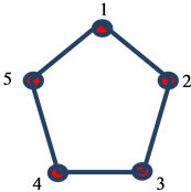
is a Circulant Graph [1] . This is C_5,2.

Our source, [1] , does not seem to state that we must have numbered vertices, but, if we do not number them, we have a polygon and there is no reason to call it Circulant. For us to have a Circulant, some sense of permutation must be passed. We then need at least the numbers there, we reckon.

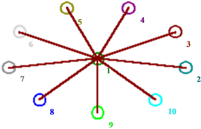
A Star Graph is [2] a tree with a central node that has degree (n − 1) and (n − 1) nodes that have degree 1. The graph below is called S₁₀.

A Starant Graph is a Circulant Graph of the type polygon with a star in the middle, so that

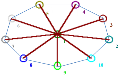
is a Starant Graph. This is SC_10,2 [3] because it has 10 nodes and 2 degrees on the circulant graph. Since a person we choose, say x, is always going to know their acquaintances, and the vertex that appears on its own in the centre of the graph would be representing this person, x, we know that the central vertex will connect to each one of the vertices of the circulant, like invariably, so that we don’t need any notation for the links between the centre and the vertices that form the circulant.

2. Development

Deterministic Small-world Communication Networks is an expression that was introduced in the scientific literature by Comellas et al. [4] as a consequence of Comellas et al. being a precursor group in terms of dealing with static pictures of selected possibilities of configuration of the communication networks. Before they do that, communication networks were seen under the light of Statistics.

As a result of playing with their results and extending them, we suggested two little refinements in their theory (what they had up to 2002), and those refinements are found in [5] .

One of those refinements was the limitation of the variable δ, which represented degrees in their work. Basically, we found a counter-example to their theory (C_9,8 with nodes 1 and 2, for instance, and C_9,6 with nodes 1 and 4) and we then had to impose a limitation on the degrees (δ ≤ 2n/3).

We also did not like the name small worlds for circulant graphs of more than 64 vertices. We don’t think that Milgram [6] associated the term with a network that could be perfectly described by a circulant of 296 vertices, but that he used the term to describe 64 subnetworks formed from that initial network of 297 vertices. We also think that these 64 subnetworks had very few vertices, something like less than ten (5.2 plus 2).

Notwithstanding, the initial assumption was actually that each vertex would connect exclusively to Milgram, never to any other vertex. The assumption was then that it was a Star Graph, not a Circulant Graph. The clustering would also be really low in this case, not high. We are here talking about the departure point.

Before the experiment begins, that is the picture. After it runs, we understand that at least 64 people connected to the others, and it is assumed that these people they connected to were unknown to them initially, in a quick way. That is 64 people out of 296, and, even so, they do not necessarily connect through someone in the initial Star Graph. That basically means that, from starters, a small world network should be something of at most 64 vertices.

Because we understand that the intentions of Comellas et al. were to mathematicise the Small World Theory, which initially belonged to Milgram, and therefore to Psychology, and we totally embrace this aim, our definitions should be exclusively mathematical.

If they are mathematical definitions, we should have a rigid limit for both the number of vertices and the amount of clustering.

Small World Networks should be networks of at most 64 nodes or should be defined in terms of ratio (64 to 296) and subnetworks, so that we respect the work of Milgram (1969).

The definitions we see online ( [7] , for instance) seem to be to the side of the proportion.

Comellas et al. define them as being something introduced by Watts and Strogatz [7] . We do observe that Milgram perhaps talked about Small World Phenomenon and Watts and Strogatz could then have talked about something different, Small World Networks.

There could be a psychological meaning to the term and it all could just imply a small group of people in our so large race, for instance.

Comellas et al. mentions the network of actors and disease spread [7] . Disease spread is a very broad topic. We could have disease spread that happens in communities that do not practice sexual disloyalty or in communities that are completely faithful to their official partners: Whilst a flu could pass quickly from one member to another, a sexual disease could die on the couple that brought it from travelling somewhere and sleeping where it was dirty. In this case, we have an isolated point, which is the couple, in a society that is likely to be formed of isolated points, which are each one of the couples, if nobody can catch the disease from anything else apart from fabric that has been in the sexual parts of another that has the disease. Clustering is really low and the number of vertices might be anything. If we talk about flu, however, everyone connects to everyone else, more than likely, so that we are now talking about a complete Starant Graph, more than likely.

If Watts and Strogratz had, as Comellas et al. seem to be suggesting, referred to both disease spread and network of actors as Small World Networks, then we would not know what to do from any of the two possible selected perspectives, it seems.

If Watts and Strogatz had, however, done the same as Milgram and worried about how two randomly chosen actors connect in terms of working together or how one disease goes from subject X to subject Y, both mentioned by the name, then we would know that his small world networks coincided with those of Milgram. In this case, they did not introduce the small world networks to us, Milgram did. We do believe that Watts and Strogatz did the same as Milgram.

Upon reading the work of Watts and Strogatz [7] , we felt like applying all to disease spread.

Their model did not seem to be good enough to describe human networks in the case of disease spread because circulant graphs usually did not have a central or main node, but we felt that diseases were spread from one individual to everyone else that formed their acquaintanceship or contact circle, so that each individual who is classified as a vector would have to be the main or central point in the social network where we study the spread.

To translate this idea into a graph, we needed to create our Starant Graph. This happened in [5] (work done in 2002).

We now could call the center Asha instead of 1 and each one of the vertices the name of a person Asha would have contact with during her day instead of 2, …, 10.

Advantages of this model over the previous model when it comes to describing human networks for the purposes of analysing disease spread:

1) There are no doubts that all that matters in disease spread is isolating the vectors, so that they are the main concern. The dot in the middle will then always, invariably, represent the vector of the disease. Because this always happens in disease spread, we’d better make our graphs be permanently like that.

2) The vector will always connect to all those they have contact with for the purposes of disease spread in a direct way, so that there is always at least and at most one edge between them and the star does the job of showing that graphically, so that the star will also always appear in the description of the network cell in the case of disease spread.

3) It is possible that the vertices, taking away the root, do not connect to each other, since it is possible that Asha sees Peter every day, say Peter is her husband and lives with her, and etc., but Peter never sees Paul, who is her boss. In fact, it is possible that he has never met him. In this case, the edges that connect the Circulant Graph could be missing. We now have a Star Graph or an SC_5,0:

It is possible, however, that each person Asha meets during her day connects to all the others, so that the graph describing her disease spread network could look like the graph below. This is an SC_5,4.

With the previous model, we would have to say that we had a Star Graph and a Complete Circulant Graph and our symbols would then be S₅ and C_5,4. We would then have to say that we have a C_5,4 together with S₅, so that we cannot even refer to the object properly. Our name and symbols save us time and make things much clearer.

4) Calculations will also be made much easier with our model, since we now will not have to analyse case by case: We can have previously calculated results for each type of Starant. That can save us a lot of time and space in the disk.

5) When we amplify the model and think about the acquaintances of Paul, for instance, we can clearly identify a repetition of patterns, but, in the past, because there was no special place for the vector, we could have to start from scratch, new calculations, different reasoning, so that our model simplifies the calculations also in the case of networks of networks, what has to save enormous amount of time and disk space.

6) It falls perfectly well inside of the idea of Milgram, Travers, Watts, and Strogatz: short characteristic path length and high clustering. With this, it is also a more adequate representation of the idea of them all, small worlds.

3. Conclusions

We conclude that the Starant Graph, a mix between a Criculant Graph and a Star Graph, is the best cell model for a human network in the case of the study of disease spread: it describes the network better, saves us time, is closer to the vision of the previous researchers in terms of the concept of Small World than the Circulant Graph is, and allows us to finally have adequate notation, suitable to scientific writing, when working with disease spread.

The symbols used to describe such a graph seem to be the best.

The work done by us should not have any intersection with the work done by Comellas et al. due to the objectives and models involved.

Small World Networks should be networks of at most 64 nodes or should be defined in terms of ratio (64 to 296) and subnetworks, so that we respect the work of Milgram (1969).

The definitions we see online ( [8] , for instance) seem to be to the side of the proportion.

Small World Networks were introduced by Milgram in 1969 [6] , not by Watts and Strogratz [7] .

Cite this paper

MarciaPinheiro, (2016) Starants: A New Model for Human Networks. Applied Mathematics,07,267-271. doi: 10.4236/am.2016.73024

References

- 1. Weisstein, E.W. (2015) Circulant Graph.
http://mathworld.wolfram.com/CirculantGraph.html - 2. Weisstein, E.W. (2015) Star Graph.
http://mathworld.wolfram.com/StarGraph.html - 3. Pinheiro, M.R. (2012) Starants II. Asian Journal of Current Engineering, 1, 259-265.
- 4. Comellas, F., Peters, J.G. and Ozon, J. (2000) Deterministic Small-World Communication Networks. Information Processing Letters, 76, 83-90.
http://dx.doi.org/10.1016/S0020-0190(00)00118-6 - 5. Pinheiro, M.R. (2007) Medium World Theories I. Applied Mathematics and Computation, 188, 1061-1070.
http://dx.doi.org/10.1016/j.amc.2006.05.213 - 6. Milgram, S. and Travers, J. (1969) An Experimental Study of the Small World Problem. Sociometry, 32, 425-443.
- 7. Strogatz, S.H. and Watts, D.J. (1998) Collective Dynamics of Small World Networks. Nature, 393, 440-442.
http://dx.doi.org/10.1038/30918 - 8. Telesford, Q.K., Joyce, K.E., Hayasaka, S., Burdette, J.H. and Laurienti, P.J. (2011) The Ubiquity of Small-World Networks. Brain Connect, 1, 367-375.
http://dx.doi.org/10.1089/brain.2011.0038