Received 25 April 2015; accepted 20 September 2015; published 23 September 2015

ABSTRACT

In this article, we give a new proof of the Itô formula for some integral processes related to the space-time Lévy noise introduced in [1] [2] as an alternative for the Gaussian white noise perturbing an SPDE. We discuss two applications of this result, which are useful in the study of SPDEs driven by a space-time Lévy noise with finite variance: a maximal inequality for the p-th moment of the stochastic integral, and the Itô representation theorem leading to a chaos expansion similar to the Gaussian case.

Keywords:

Lévy Processes, Poisson Random Measure, Stochastic Integral, Itô Formula, Itô Representation Theorem

1. Introduction

Random processes indexed by sets in the space-time domain are useful objects in stochastic analysis, since they can be viewed as mathematical models for the noise perturbing a stochastic partial differential equation (SPDE). In the recent years, a lot of effort has been dedicated to studying the behaviour of the solution of basic equations (like the heat or wave equations), driven by a Gaussian white noise. This type of noise was introduced by Walsh in [3] and is defined as a zero-mean Gaussian process, with covariance

, where denotes the Lebesgue measure and is the class of bounded

Borel sets in.

In the recent articles [1] [2] , a new process has been introduced as an alternative for the Gaussian white noise perturbing an SPDE, which has a structure similar to a Lévy process. We introduce briefly the definition of this process below.

Let N be a Poisson random measure (PRM) on of intensity where and is a Lévy measure on:

We denote by the compensated PRM defined by for any Borel set A in with. The Lévy-type noise process mentioned above is defined as, where

for some. It was shown in [2] that Z is an “independently scattered random measure” (in the sense of [4] ) with characteristic function:

(In particular, Z can be an a-stable random measure with, as in Definition 3.3.1 of [5] .) One can define the stochastic integral of a process with respect to Z and for a certain integrands,

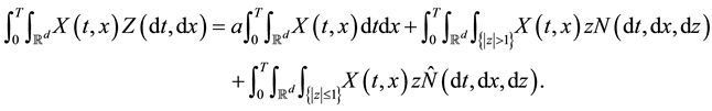
The stochastic integral with respect to (or N) can be defined using classical methods (see e.g. [6] ). We review briefly this definition here.

Assume that N is defined on a probability space. On this space, we consider the filtration

where is the class of bounded Borel sets in and is the class of Borel sets in which are bounded away from 0.

An elementary process on is a process of the form

where, X is an -measurable bounded random variable, and. A pro- cess is called predictable if it is measurable with respect to the s-field

generated by all linear combinations of elementary processes.

As in the classical theory, for any predictable process H such that

(1)

we can define the stochastic integral of H with respect to and the process

is a zero-mean square-integrable martingale which satisfies

(2)

On the other hand, for any predictable process K such that

we can define the integral of K with respect to N and this integral satisfies

(3)

In this article, we work with processes whose trajectories are right-continuous with left limits. If x is a right

continuous function with left limits, we denote by the left limit at time t and

the jump size at time t. We will prove the following result.

Theorem 1 (Ito Formula I). Let be a process defined by

(4)

where G, K and H are predictable processes which satisfy

(5)

(6)

(7)

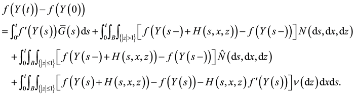
Then there exists a modification of Y (denoted also by Y) whose sample paths are right-continuous with left limits, such that for any function and for any, with probability 1,

(8)

Note that since the first two terms on the right-hand side of (4) are processes of finite variation and the last term is a square-integrable martingale, Y is a semimartingale. Therefore, the Itô formula given by Theorem 1 can be derived from the corresponding result for a general semimartingale, assuming that Y has sample paths which are right-continuous with left limits (see e.g. Theorem 2.5 of [7] ).

The goal of the present article is to give an alternative proof of this result which contains the explicit construction of the modification of Y for which the Itô formula holds.

We will also give the proof of the following variant of the Itô formula, which will be useful for the applications related to the (finite-variance) Lévy white noise, discussed in Section 4.

Theorem 2 (Ito Formula II). Let be a process defined by

(9)

where G and H are predictable processes which satisfy (5), respectively (1). Then there exists a càdlàg modification of Y (denoted also by Y) such that for any, with probability 1,

The method that we use for proving Theorems 1 and 2 is similar to the one described in Section 4.4.2 of [6] in the case of classical Lévy processes, the difference being that in our case, N is a PRM on instead of. This method relies on a double “interlacing” technique, which consists in first approximating the set of small jumps by sets of the form with (in the case when H and K vanish outside a bounded Borel set), and then approximating the spatial domain by regions of the form with. This approximation method is described in Section 2. Section 3 is dedicated to the proofs of Theorems 1 and 2. Finally, in Section 4 we discuss two applications of Theorem 2 in the case of the (finite-variance) Lévy white noise introduced in [1] .

2. Approximation by Right-Continuous Processes with Left Limits

In this section, we show that the Lévy-type integral processes given by (4) and (9) have right-continuous modifications with left limits, which are constructed by approximation. These modifications will play an important role in the proof of Itô’s formula. Since the process is continuous, we assume that.

We consider first processes of the form (4). We start by examining the case when both integrands H and K

vanish outside a set. Since the process is clearly càdlàg

(the integral being a sum with finitely many terms), we need to consider only the integral process which depends on H.

Note that if H vanishes a.e. on for some and, then

is a process whose sample paths are right-continuous with left limits (the first term is a sum with finitely many terms and the second term in continuous). Therefore, we will suppose that H satisfies the following assumption:

Assumption A. It is not possible to find and such that

with respect to the measure.

Lemma 1. Let be a process defined by

where and H is a predictable process which satisfies Assumption A and

(10)

Then, there exists a càdlàg modification of Y such that for all,

where

for some sequence (depending on T) such that.

Proof: We use the same argument as in the proof of Theorem 4.3.4 of [6] . Fix. Let

where

Note that is non-increasing and. (If then for all n. Hence, which contradicts Assumption A.)

Note that is a càdlàg martingale. By Doob’s submartingale inequality and relation (2),

By Chebyshev’s inequality,. By Borel-Cantelli lemma, with probability 1, the sequence is Cauchy in the space of càdlàg functions on equipped with the sup-norm. Its limit is a modification of Y since for any, also converges to in. Finally, we note that the process does not depend on T (although the approximation sequence does). If is the modification of Y on and is the modification of Y on with, then a.s. for any. Hence, can be extended to. ,

We consider now the case when the at least one of the integrands H and K do not vanish outside a set. More precisely, we introduce the following assumptions:

Assumption B. It is not possible to find and such that

with respect to the measure.

Assumption. It is not possible to find and such that

with respect to the measure.

We consider bounded Borel sets in of the form.

Theorem 3 (Interlacing I). Let be a process defined by (4) with, where H and K are predictable processes which satisfy conditions (7), respectively (6), such that either H satisfies Assumption B, or K satisfies Assumption. Then, there exists a càdlàg modification of Y such that for all T > 0,

(11)

where is a càdlàg modification of the process defined by

with for some sequence (depending on T) such that.

Proof: Fix. Let where

Note that is non-decreasing and. (If then for all n, and hence, which contradicts Assumptions B or.) Let be the process given in the statement of the theorem with. We denote by and the two integrals which compose, depending on H, respectively K.

We denote by the càdlàg modification of given by Lemma 1. By Doob’s submartingale inequality and relation (2),

By Chebyshev’s inequality,.

Note that is a càdlàg process. For any,

and hence, using relation (3),

By Markov’s inequality,.

Let. Then, and the conclusion follows by the Borel-Cantelli Lemma, as in the proof of Lemma 1. ,

We consider next processes of the form (9) with G = 0. Note that if H vanishes a.e. outside a set then

where the first term has a càdlàg modification given by Lemma 1, the second term is càdlàg, and the third term is continuous. Therefore, we will suppose that H satisfies the following assumption:

Assumption C. It is not possible to find and such that

with respect to the measure.

Theorem 4 (Interlacing II). Let Y be a process given by (9) with, where H is a predictable process which satisfies (1) and Assumption C. Then, there exists a càdlàg modification of Y such that (11) holds, where is a càdlàg modification of the process defined by:

with for some sequence (depending on T) such that.

Proof: We proceed as in the proof of Theorem 3. Fix. Let where

By Assumption C,. We write Y_n(t) as the sum of two integrals, corresponding to the regions,

and. We denote these integrals by, respectively. Note that is càdlàg. Let

be the càdlàg modification of given by Lemma 1.

Let. By Doob’s submartingale inequality,

and the conclusion follows as in the proof of Lemma 1. ,

3. Proof of Itô Formula

In this section, we give the proofs of Theorem 1 and Theorem 2.

We start with the simpler case when there are no small jumps (the analogue of Lemma 4.4.6 of [6] ).

Lemma 2. Let

where G is a predictable process which satisfies (5), , and K is a predictable process. Then, for any function and for any,

Proof: We denote. By Proposition 5.3 of [8] , we may assume that the restriction of N to the set has points, where are the points of a Poisson process on of intensity and are i.i.d. on with distribution, independent of. We consider two cases.

Case 1: G = 0. By the representation of N,. So is a step function which has a jump of size at each point and. Hence

and the conclusion follows since N has points in.

Case 2: G is arbitrary. The map is a step function which has a jump of size at time. Since is continuous, the jump times and the jump sizes of Y coincide with those of, i.e.. We use the decomposition

where A and B are defined as follows: if, we let

Note that

It remains to prove that

(12)

For this, we assume that and we write

So it suffices to prove that

(13)

for all, and

(14)

We first prove (13). Fix. For any

, and.

We extend by continuity to. Hence

where for the last equality we used the fact that and hence

.

This proves (13).

Next, we prove (14). Note that if, both terms are zero. So, we assume that. For any

, and.

Arguing as above, we see that

where for the last equality we used the fact that and hence

.

This concludes the proof of (14). ,

Proof of Theorem 1: We fix. We assume that and are bounded. (Otherwise, we use for.)

Case 1: H and K vanish outside a fixed set.

If H vanishes a.e. on for some and, the conclusion follows from Lemma 2. Therefore, we suppose that H satisfies Assumption A. By Lemma 1, there exists a càdlàg modification of Y (denoted also by Y) such that

(15)

where the process is defined by

being the sequence given by Lemma 1 with. Consequently,

(16)

Note that

where and. By the

Cauchy-Schwarz inequality, satisfies (5) (since B is a bounded set and H satisfies (10)). We apply Lemma 2 to:

After using the definitions of and, as well as adding and subtracting

we obtain that:

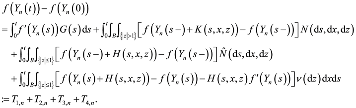(17)

We denote by, respectively the four terms on the right-hand side of (8). The conclusion will follow by taking the limit as in (17). The left-hand side converges to, by (15).

We treat separately the four terms in the right-hand side. By the dominated convergence theorem,

Since is a sum with a finite number of terms, using (15) and the continuity of f, we see that a.s. For the third term, note that, where

and a.s., by (15) and the continuity of f. By the dominated convergence theorem, and. To justify the application of this theorem, we use Taylor’s formula of the first order:

(18)

and the fact that is bounded. This proves that in.

Finally, , where

and

a.s., by (16) and the continuity of f. By the dominated convergence theorem, and. To justify the application of this theorem, we use Taylor’s formula of second order:

(19)

and the fact that is bounded. This proves that in.

Case 2. H satisfies Assumption B or K satisfies Assumption.

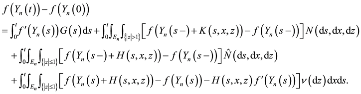
By Theorem 3, there exists a càdlàg approximation of Y (denoted also by Y) such that (15) holds, where is a càdlàg modification of

being the sequence given by Theorem 3 with. Using the result of Case 1 for the pro- cess, we obtain

The conclusion follows letting as in Case 1. ,

Proof of Theorem 2: We assume that and are bounded. We fix t.

Case 1. H vanishes outside a set. We write

where. By the Cauchy-Schwarz inequality, satisfies (5) (since B

is a bounded set). By Theorem 1, there exists a càdlàg modification of Y (denoted also by Y) such that

We add and subtract. The conclusion follows by rear-

ranging the terms.

Case 2. H satisfies Assumption C.

By Theorem 4, there exists a càdlàg modification of Y (denoted also by Y) such that (15) holds, where is a càdlàg modification of

being the sequence given by Theorem 4 with. We write the Itô formula for the process (using Case 1) and we let. ,

4. Applications

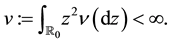
In this section, we assume that the Lévy measure satisfies the condition:

As in [1] , we consider the process defined by:

For any predictable process such that

(20)

we can define the stochastic integral of X with respect to L and this integral satisfies:

By (2), this integral has the following isometry property:

When used as a noise process perturbing an SPDE, L behaves very similarly to the Gaussian white noise. For this reason, L was called a Lévy white noise in [1] .

4.1. Kunita Inequality

The following maximal inequality is due to Kunita (see Theorem 2.11 of [7] ). In problems related to SPDEs with noise L, this result plays the same role as the Burkholder-Davis-Gundy inequality for SPDEs with Gaussian white noise.

Theorem 5 (Kunita Inequality). Let be a process given by

where X is a predictable process which satisfies (20).

If for some, then for any,

where and is the constant in Theorem 2.11 of [7] .

Proof: We apply Theorem 2 with and. The proof is identical to that of Theorem 2.11 of [7] . We omit the details. ,

Remark 1. Kunita’s constant cannot be computed explicitly. Theorem 5 is proved in [9] using a different method which shows that is directly related to the constant in Rosenthal’s inequality, which is.

4.2. Itô Representation Theorem and Chaos Expansion

In this section, we give an application to Theorem 2 to exponential martingales, which leads to Itô representation theorem and a chaos expansion (similarly to Sections 5.3 and 5.4 of [6] ).

For any we let for. We work with the càdlàg modi-

fication of the process given by Theorem 4. By Lemma 2.4 of [1] ,

where

Hence for all, where

The following result is the analogue of Lemma 5.3.3 of [6] .

Lemma 3. For any and, with probability 1,

Proof: We apply Theorem 2 to the function and the process

Hence, and. We obtain:

Since the sum of the last two integrals is 0, the conclusion follows. ,

We fix. We let. We denote by be the space

of C-valued square-integrable random variables which are measurable with respect to.

Lemma 4. The linear span of the set is dense in.

Proof: The proof is similar to that of Lemma 5.3.4 of [6] . We omit the details. ,

Theorem 6 (Ito Representation Theorem). For any, there exists a unique predictable C-valued process satisfying

(21)

such that

(22)

Proof: By Lemma 3, relation (22) holds for with. The conclusion follows by an approximation argument using Lemma 4. ,

The multiple (and iterated) integral with respect can be defined similarly to the Gaussian white-noise case (see e.g. Section 5.4 of [6] ).

More precisely, we consider the Hilbert space, where

, and.

For any integer, we consider the n-th tensor product space. The n-th multiple integral with respect to can be constructed for any function, and this integral has the isometry property:

Moreover, if, then for all and.

We have the following result.

Theorem 7 (Chaos Expansion). For any, there exist some symmetric functions, such that

In particular,

Proof: We use the same argument as in the classical case, when is a PRM on and

is a square-integrable Lévy process (see Theorem 5.4.6 of [6] or Theorem 10.2 of [10] ). By Theorem 6, there exists a predictable process satisfying (1) such that

(23)

By (21), for almost all. For such fixed, we apply Theorem 6 again to the variable. Hence, there exists a predictable process

Satisfying

such that

We substitute this into (23) and iterate the procedure. We omit the details. ,

Acknowledgements

Research of R. M. Balan is funded by a grant from the Natural Sciences and Engineering Research Council of Canada.

Cite this paper

Raluca M.Balan,Cheikh B.Ndongo, (2015) Itô Formula for Integral Processes Related to Space-Time Lévy Noise. Applied Mathematics,06,1755-1768. doi: 10.4236/am.2015.610156

References

NOTES

^*Corresponding author.

References

- 1. Balan, R.M. (2015) Integration with Respect to Lévy Colored Noise, with Applications to SPDEs. Stochastics, 87, 363- 381.
http://dx.doi.org/10.1080/17442508.2014.956103 - 2. Balan, R.M. (2014) SPDEs with α-Stable Lévy Noise: A Random Field Approach. International Journal of Stochastic Analysis, 2014, Article ID: 793275.
http://dx.doi.org/10.1155/2014/793275 - 3. Walsh, J.B. (1989) An Introduction to Stochastic Partial Differential Equations. Ecole d’Eté de Probabilités de Saint- Flour XIV. Lecture Notes in Math, 1180, 265-439.
http://dx.doi.org/10.1007/BFb0074920 - 4. Rajput, B.S. and Rosinski, J. (1989) Spectral Representations of Infinitely Divisible Processes. Probability Theory and Related Fields, 82, 451-487.
http://dx.doi.org/10.1007/BF00339998 - 5. Samorodnitsky, G. and Taqqu, M.S. (1994) Stable Non-Gaussian Random Processes. Chapman and Hall, New York.
- 6. Applebaum, D. (2009) Lévy Processes and Stochastic Calculus. 2nd Edition, Cambridge University Press, Cambridge.
http://dx.doi.org/10.1017/CBO9780511809781 - 7. Kunita, H. (2004) Stochastic Differential Equations Based on Lévy Processes and Stochastic Flows of Diffeomorphisms. In: Rao, M.M., Ed., Real and Stochastic Analysis, New Perspectives, Birkhaüser, Boston, 305-375.
http://dx.doi.org/10.1007/978-1-4612-2054-1_6 - 8. Resnick, S.I. (2007) Heavy Tail Phenomena: Probabilistic and Statistical Modelling. Springer, New York.
- 9. Balan, R.M. and Ndongo, C.B. (2015) Intermittency for the Wave Equation with Lévy White Noise. Arxiv: 1505.04167.
- 10. Di Nunno, G., Oksendal, B. and Proske, F. (2009) Malliavin Calculus for Lévy Processes with Applications to Finance. Springer-Verlag, Berlin.
http://dx.doi.org/10.1007/978-3-540-78572-9