Applied Mathematics
Vol.5 No.2(2014), Article ID:42172,18 pages DOI:10.4236/am.2014.52031
Finding and Choosing among Multiple Optima
1Department of Applied Mathematics and Statistics, University of California, Santa Cruz, USA
2Quantitative Modeling and Analysis, Sandia National Laboratories, Livermore, USA
Email: jguenthe@soe.ucsc.edu, herbie@ams.ucsc.edu, gagray@sandia.gov
Received November 12, 2013; revised December 12, 2013; accepted December 19, 2013
ABSTRACT
Black box functions, such as computer experiments, often have multiple optima over the input space of the objective function. While traditional optimization routines focus on finding a single best optimum, we sometimes want to consider the relative merits of multiple optima. First we need a search algorithm that can identify multiple local optima. Then we consider that blindly choosing the global optimum may not always be best. In some cases, the global optimum may not be robust to small deviations in the inputs, which could lead to output values far from the optimum. In those cases, it would be better to choose a slightly less extreme optimum that allows for input deviation with small change in the output; such an optimum would be considered more robust. We use a Bayesian decision theoretic approach to develop a utility function for selecting among multiple optima.
Keywords:Bayesian Statistics; Treed Gaussian Process; Emulator; Decision Theory; Optimization
1. Introduction
Optimization traditionally focuses on just finding the most extreme value, such as a global minimum. However, there are many cases where one wants a robust answer, such that a small change in the inputs will not lead to a large change in the outputs and thus a result far from the original optimum. Two common examples are situations where there is the potential for users not to be precise about the input, or where there is uncertainty in the parameters. An example of the first is developing a recipe, where you want the resulting food to taste very good, but need to realize that not everyone following the recipe will measure all quantities exactly, and thus it is important for small deviations from the recipe to lead to nearly equivalent results. One wants an optimum that allows for small deviations even if its value is not quite as extreme, rather than an optimum with a more extreme value that becomes much less extreme with small deviations (a “knife’s edge”). An example of the second is our application in Section 6 of a groundwater contamination remediation problem, where wells will be drilled to prevent contamination from entering a nearby river. It is important that the result be similar even if the wells are not drilled exactly as specified, or if the hydraulic heads that appear in reality are not quite the same as predicted in theory.
This paper considers the problem of finding the best optimum in derivative-free optimization, where we take into account not just the extremal value, but also the robustness of the result, as measured by several factors. First, we develop a search algorithm using statistical modeling to emulate the objective function, taking a more global perspective, and hybridize it with a local direct optimization method, one that is provably convergent to a local optimum. Once promising modes have been found, we use a Bayesian decision theoretic framework, defining a utility function to account for different aspects of robustness. Without loss of generality, we focus on minimization, as maximization can be obtained by minimizing the negative of the function. We generally favor an optimum where the function is relatively smooth, as opposed to a spiky optimum. For example, we consider the two quadratic functions in Figure 1 with univariate input x and univariate output y, where one has a lower minimum but more curvature, and the other is rather flat. The two vertical lines denote a local region around the minima of each curve. While the function with higher curvature has the lower minimum, it mostly falls above the other curve in the local region. Thus we might prefer the more flat curve, as it has a lower average value over the local region, and it never rises far above its minimum value in the region; it is more robust as a minimum.
Some related approaches in the literature are Pareto-based ranking schemes utilized in multi-objective optimization [1,2], and techniques established in global search heuristic optimization methods such as genetic algorithms [3-5] and particle swarm optimization [6]. We emphasize that a critical difference in our approach is that we want to consider a set of optima, while existing methods in the literature are focused on finding a single best optimum, or the best optimum for each of several attributes. While other methods can identify multiple optima as part of their search routine, there is no explicit attempt to find minima which are not the global minimum, and thus promising local minima could remain unexplored. Here we develop a new approach based on statistical emulation for searching the space and identifying multiple minima, and then use Bayesian decision theory to choose among those minima. Emulation uses a statistical model to estimate the objective function at unobserved points, when the function is expensive to evaluate and so we only have limited observations. In this paper, we consider the function to be deterministic, i.e., there is no noise or stochasticity in the function evaluations. The standard statistical model for emulation is the Gaussian process, a computationally accessible nonparametric model that can accommodate a range of response functions [7]. An improvement over the traditional Gaussian process is the treed Gaussian process (TGP), which has the capability of modeling functions with regions of different variability (nonstationarity) better than a stationary Gaussian process [8], and we use TGP as our emulator throughout this paper. Fitting the emulator in a Bayesian framework allows for full accounting of uncertainty. Uncertainty in predicting the function output values is captured by the posterior predictive distribution [9], which gives a probability distribution of the possible output values for each unobserved input. Combining the posterior predictive with a Bayesian decision theory framework allows us to incorporate the uncertainty in the function outputs into our optimal decision.
2. Searching for Multiple Optima
Many functions of interest, such as black-box computer simulator functions, often have several optima. In this section we develop an algorithm that explores the input space to find all significant optimum candidates in order
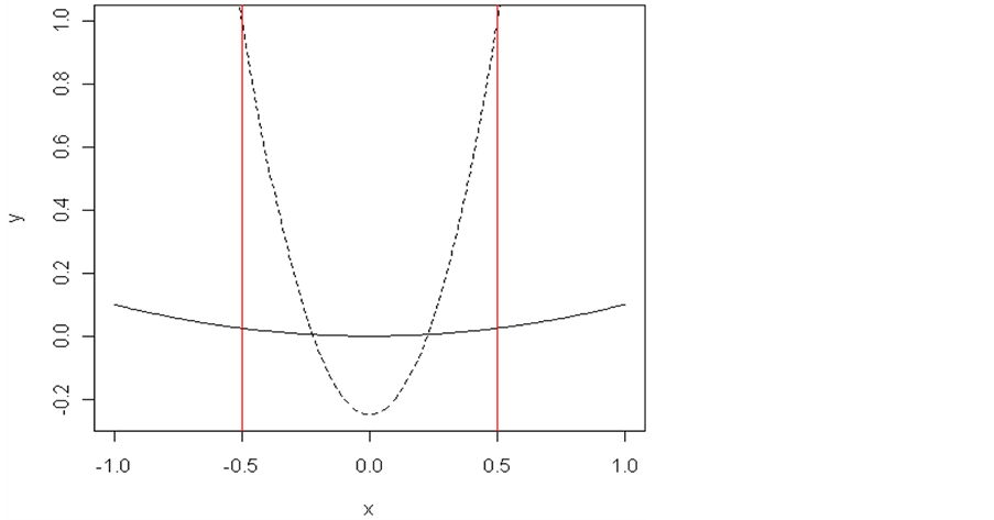
Figure 1. Robustness illustration on two minima superimposed at the origin for visualization. The two vertical red lines denote a local region of interest. Although the minimum with more curvature has a lower function value, the smoother minimum has a lower mean value in the region and it does not move far from the minimum value in the region.
to select those most suitable. Our approach was inspired by several articles on optimization [10-]">]">12]. A critical underlying idea is that of expected improvement [13]. The improvement function is defined as  where
where  is the minimum value of the training points,
  is the true (but as yet unobserved) output value for input point
![]() , and
, and ![]() designates the input space. Thus there is only “improvement” if we find a new point with a smaller output than our best observed point so far. Because the truth is unknown without evaluating the function, we use our statistical emulator to get a prediction, or in the Bayesian framework, a full posterior predictive distribution for
designates the input space. Thus there is only “improvement” if we find a new point with a smaller output than our best observed point so far. Because the truth is unknown without evaluating the function, we use our statistical emulator to get a prediction, or in the Bayesian framework, a full posterior predictive distribution for . The expected improvement,
  is the expectation of the improvement function with respect to the posterior predictive distribution. The expected improvement balances favoring points whose predicted values are small with points whose predicted values may be less small but whose uncertainty in the prediction is large, and thus we realize that there is a certain probability that that point could be a new minimum. One minimization approach [13] is to iteratively choose the next function evaluation to be the point that maximizes the expected improvement. [10,]">]">12] illustrate how to guide the search for optima using a TGP emulator and the statistic for maximum expected improvement. The diagnostics discussed in [11] led to the use of the errors and standardized errors of adaptively sampled points for verifying the emulator model.
We use a hybrid optimization approach, similar to [10], in which we combine statistical emulation with a provably convergent local direct search method. Here we use pattern search [14], although other approaches such as trust region optimization [15, for example] could be used. The statistical model takes a more global and exploratory perspective, while the direct method quickly hones in on each local minimum. We leverage the convergence of the direct method by attempting to start it where it will converge to a new minimum rather than a previously explored one.
Our algorithm proceeds as follows: The objective function is modeled by the emulator within the designated input space. This surface can be thought of as a two dimensional surface with “hills”, “valleys”, and “plains”. Our concern is with the “valleys” since they encompass the minimum points. Although the emulator surface differs from the true function to some degree, it is expected to have increasingly close correspondence as we obtain more function evaluations. Starting from a promising minimum point on the emulator surface, pattern search is provably convergent to a local minimum of the objective function. Once a minimum has been found, the search region for other minima is restricted to avoid re-targeting the known minimum. This region is defined initially by a boundary at distance ![]() from the known minimum. To find
from the known minimum. To find![]() , we compute the distance of each predicted point to the known minimum, and then find the maximum,
, we compute the distance of each predicted point to the known minimum, and then find the maximum,  , of these distances. Let
 . Only predicted points that are this distance or greater from the known minimum are starting point candidates for the next search. This distance may be adjusted so that the minimum predicted point in this region has a value nearly equal to or just less than a limiting value as given by the user. (Since the predicted points are a discrete set, contiguous points may overlap this limiting value). Minima with optimal values above this limiting value are not of interest. With each new minimum found by pattern search, the search region changes to exclude this minimum by updating
  to account for the new minimum, and the updating
 ![]() and the search region. After all minima less than or approximately equal to the limiting value are found, the search process is ended and each minimum is evaluated for its utility (or significance) by the optimum selection utility, as described in Section 3.
and the search region. After all minima less than or approximately equal to the limiting value are found, the search process is ended and each minimum is evaluated for its utility (or significance) by the optimum selection utility, as described in Section 3.
A user must decide to what level, relative to the global minimum and the mean value, the search is to be extended. Let the global minimum be  and the expected mean value of the objective function be approximated by the mean value
  of the emulator model predicted points. We want to find local minima whose values are not too far above the global minimum. A ratio
 ,
, ![]() , is chosen where
, is chosen where . The upper bound
  is computed from the current observed “global” minimum and
  value by
 . While the actual value of
  may not yet be known, the lowest value among the current minima is used for
 .
.  becomes a better approximation to the actual mean value of the objective function in the input region as the minima search progresses.
For each stage of the algorithm, the emulator (our treed Gaussian process) uses the current training point set to predict a large random sample at new input points. The first minimum is found by using the minimum value obtained from the emulator model to initiate a run of a local direct optimization routine (pattern search). As the algorithm proceeds, the new function evaluations are added to the training point set. At the first stage, we use the one minimum value as the initial , while in future stages, we use the smallest observed
 ![]() as
as .
.
We determine ![]() as above and thus define the search region, then use the emulator to predict the minimum point in the search region by evaluating a large sample of candidate input points in the search region. Denote predicted minimum value by
as above and thus define the search region, then use the emulator to predict the minimum point in the search region by evaluating a large sample of candidate input points in the search region. Denote predicted minimum value by . There are two cases: 1) The minimum predicted point value,
  , is less than the desired upper bound
 ; 2)
; 2) .
.
For the first case,  , so there is potential for finding a new local minimum, but we also want to be sure that it is a new minimum, rather than running a local search and converging back to our already known minimum. To see if this new point is in a different zone of attraction, we look for a “ridge” of points that have higher values and separate the new point from the known minimum. We define a quantity
  which is the width of an interval
 , where
  is the distance from
  to the closest known minimum. The interval width
  is dependent on the sample size of the predicted points (candidate points predicted by the emulator, not the actual function evaluations). This interval must be large enough to include predicted points between the current
  point and its closest minimum. It should be chosen so that a hypercube of width
  has a high probability of including a predicted point. The smaller it can be made to include points between
  and the closest minimum, the better. However, if it is set too small, it will not be effective for determining that there is a ridge of higher values between
  and the known minima. We have found a good default value for
  to be
to be , where
  is upper bound minus the lower bound (span) of the input space,
 ![]() is the number of predicted points,
is the number of predicted points,  is the dimension of the input space, and 2 is a factor to make this interval larger than the average distance between closest predicted points. As the dimension of the input space increases, the value determined for
  increases. In cases where it is too large to be used effectively, the algorithm reverts to adjusting the search region distance until
 .
.
The lowest predicted value from candidate points in the interval  is compared to
 . If the smallest predicted value in this interval is greater than
 , then the point with value
  is associated with a minimum within the current search region and it becomes the next starting point for pattern search. The reasoning here is that there must be a “ridge” of higher predicted points between the known minima and the point with predicted value
 . Essentially, this means that a straight line path from the point with value
  to the closest minimum would pass through points having higher values than
 . In terms of a two dimensional surface having
 ![]() values representing elevations, the path would climb over a ridge or hill to get to that minimum. On the other hand, if the smallest value for the interval is less than or equal
values representing elevations, the path would climb over a ridge or hill to get to that minimum. On the other hand, if the smallest value for the interval is less than or equal , the search region distance is increased by a factor greater than 1 (e.g., 1.05). For this new region, a new
  is determined. If
 , the point with value
  becomes the next starting point for pattern search. If it is still true that
 , the procedure as described above is repeated. As successive increases are applied to the region distance, eventually either
  or the smallest valued point in the interval
  is greater than
 . In either case the next starting point for pattern search is the point with value
 . If, during increases of the region distance,
  exceeds
 , the region distance is set to the average of the last two distances, which should yield a
  approximately equal to
 . We now illustrate three different situations where
 .
.
In Figure 2, the current known minimum is shown as the blue “X” (lower left) and the minimum valued point in the search region is the red “X” (upper left). The two large black dashed circles (only a quarter of each circle fits in this figure) are the lower and upper boundaries of the interval . The red dashed circle (in between the black circles) is the current search region boundary at distance
 ![]() from the current known minimum. Here
from the current known minimum. Here . The little blue circles are a random sample of candidate predicted points in the search region and in the interval
 . The space between the two black dashed circles is representative of the “ridge” of predicted points that have higher values than the point marked with the red “X”. So the point marked with the red “X” is the starting point of the next search and should locate a minimum within the search region.
Two situations where  lies on the boundary of the search region (red dashed line) are shown in Figure 3. Consider the schematic on the left. Here the red “X” marks the point
 . The blue “X” is the known minimum and
 . If the search region boundary distance is not increased (moved out), the known minimum would be found again. However, pursuant to the algorithm logic, the search region boundary is moved out until a ridge of higher predicted values are between
  (the black “X”) and the known minimum. That occurs when the search region boundary is the black dashed line. So, increasing the search region distance when
  is effective in this situation.
Now consider the schematic on the right. The point with value  is marked with a red “X”. The known minimum is marked with a blue “X”. Again,
 . The search starting from this point would find the minimum within the −0.8 contour. However, the algorithm can not distinguish between the first situation and this second situation in Figure 3. To protect against the first situation, since there is no ridge of higher predicted
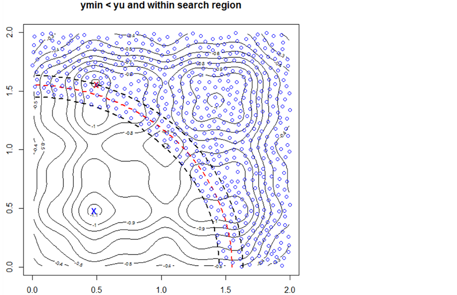
Figure 2.  and
and  Interior to the Search Region Boundary: The contour graph has the known minimum marked with a blue “X”. The boundary of the search region is the red dashed line. The point
  is marked with a red “X”. It is within the search region. To establish whether it is the next starting point for pattern search, the minimum value of the ridge of points within the blacked dashed lines of the interval
  is tested against
 . The blue “o”s represent the predicted points in this interval and the search region. The contours indicate the point
  has a value lower than this ridge of points and, as a starting point, the next minimum found should be within the small contour near
  (red “X”).
points between  and the known minimum, the algorithm increases the search region distance until
 , the point marked with a black “X”. This new point with the value
  becomes the next search point and should find the minimum within the −0.8 contour. So, moving the boundary out is effective in both situations.
For the case , our emulator is not predicting any new minima in the search region that are below our threshold of interest. Thus the search region is widened by decreasing
 ![]() by a factor less than 1 (e.g., 0.95) to include more predicted points until the predicted minimum,
by a factor less than 1 (e.g., 0.95) to include more predicted points until the predicted minimum,  in the search region is approximately equal to
 .
.
This predicted point is then used for the next search point. The adjustment of ![]() is done similarly to the case where
is done similarly to the case where . When the last decrease of
 ![]() causes
causes  to fall below
 , the search region distance becomes the average of the previous distance and the current distance. A schematic of this case is shown in Figure 4.
Here two minima are close together. The current known minimum is marked with a blue “X”. The red dashed outer circle is the initial search region boundary. It is uncertain whether starting from the initial , marked with a red “X”, will find a new minimum since the region is relatively flat. The search region boundary distance is decreased. This is shown as the inner black dashed circle. The black “X” now represents the predicted point with a value
  that approximates
 . This becomes the next search point.
For this algorithm to work, the predicted point values must be reasonable approximations to the simulator surface. If this is not the case, some minima within the upper level specified by the ratio 
 will be missed. So adaptively sampled points to improve the fit of the emulator surface are important. The starting step size used in pattern search is also very important for the algorithm. Initially, when the minima are relatively far
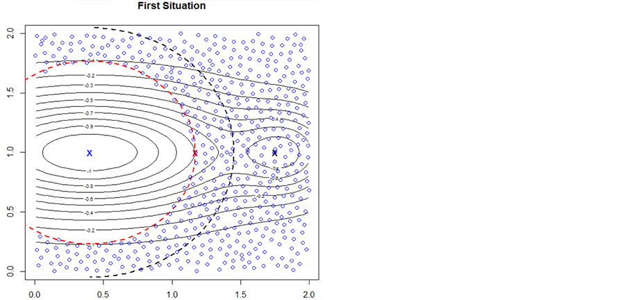
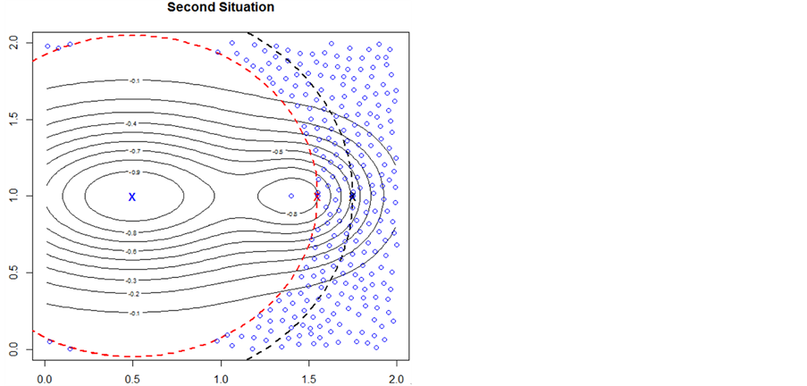
Figure 3. Two Situations where  is on the Search Region Boundary: In the schematic on the left, the red “X” marks the point
 . The blue “X” is the known minimum and
 . If the search region boundary distance is not increased (moved out), the known minimum would be found again. However, pursuant to the algorithm logic, the search region boundary is moved out until a ridge of higher predicted values are between
  (the black “X”) and the known minimum. That occurs when the search region boundary is the black dashed line. So, increasing the search region distance when
  is effective in this situation. In the schematic on the right, the point with value
  is marked with a red “X”. The known minimum is marked with a blue “X”. Again,
 . The search starting from this point would find the minimum within the −0.8 contour. However, the algorithm can not distinguish between the first situation and this second situation. To protect against the first situation, since there is no ridge of higher predicted points between
  and the known minimum, the algorithm increases the search region distance until
 , the point marked with a black “X”. This new point with the value
  becomes the next search point and should find the minimum within the −0.8 contour. So, moving the boundary out is effective in both situations.
apart, the step size should be relatively large. This is best for finding the dominant minima, since the tendency is then for pattern search to “step over” minima with smaller values and zones of attraction (the region where a hypothetical marble, if dropped, would roll toward the minimum). As the distance of search points to current minima decreases, the step size is decreased accordingly. A larger step size could find a previously found dominant minimum. The step size is chosen as a fraction  of the distance to the closest known minimum. With this smaller step size, a less dominant minimum that lies close to a known minimum is more likely to be found.
The algorithm as described above is intended to search for minima for relatively smooth objective functions with few discontinuities. The pseudo code for this algorithm is in Section 8. If the function is expected to be irregular, or to have many discontinuities, then some modifications may be required. We discuss one such approach in the context of the hydrology application in Section 6.
3. Optimum Selection Methodology
Once we have identified a set of promising minima, we can then decide which one is most useful. Optimum selection should be based on a user’s decision about what is most important in choosing a robust optimum. To be precise about optimum features, we focus our attention on a local region of interest around each optimum, referred to as a “tolerance region” or defined by the tolerance distance from the optimum to the edge of the region. For simplicity we generally use a hypercube in the input space centered at the local argmin (the input value that leads to the local minimum of the output function), but other regions could be substituted (e.g., hyperrectangles).
We consider four aspects of a local optimum: 1) the minimum value (lower bound), 2) the mean value in the
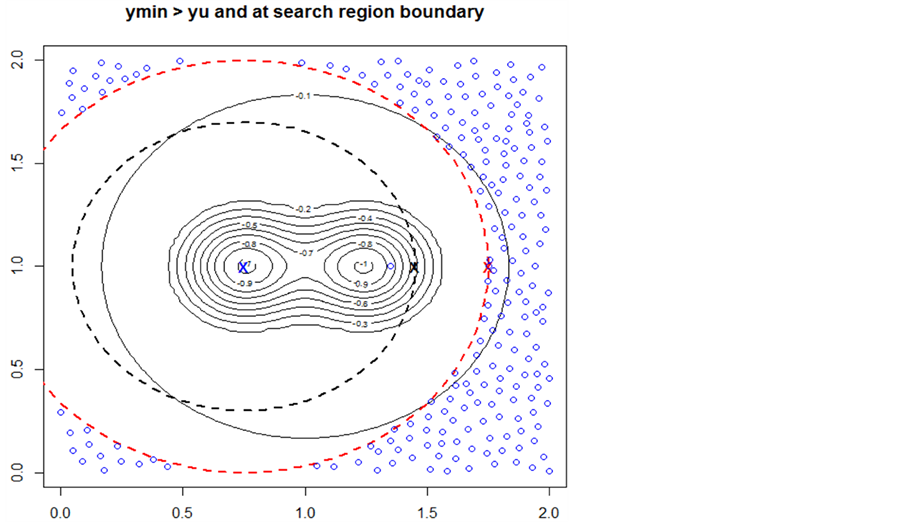
Figure 4. Minima Search for Cases where : The contour graph has the known minimum marked with a blue “X”. There is another minimum close to this known minimum indicated by the circle contours. The search region boundary is the red dashed line. The predicted points in the search region are the blue “o”s. The first
  point is marked with a red “X”. It is uncertain whether a search starting from this point
  would find the minimum close to the known minimum. Since
 , the search boundary is moved in until
 . This happens when the search boundary is the black dashed line. The new point
  becomes the point marked with the black “X”. Starting from this point the other minimum should be found.
tolerance region, 3) the maximum value in the tolerance region (upper bound), 4) the range of values (upper bound minus lower bound) in the tolerance region. Consider the three local optima from a bivariate input function shown in Figure 5.
The left column shows the histograms of the function values in each tolerance region. The right column shows the variable paths made by holding one variable constant and varying the other through the tolerance region. The minima are symmetric so these paths are the same for either variable. The blue dashed vertical line shows the global minimum value in the histograms and the horizontal blue dashed lines show the global minimum value in the variable paths. The vertical red solid line shows the mean output value in each tolerance region. There are reasons to consider each of these minima:
• The first minimum might be chosen since it has the lowest upper bound and the least variation. The lowest upper bound is important since, in choosing this minimum, the user can depend on having a value no more than this upper bound. Also, the small range demonstrates that the values in the tolerance region vary the least.
• The second minimum might be chosen since it has the lowest average (solid red line), indicating good performance in minimization across the region.
• The third minimum might be chosen since it has the lowest value (it is the global minimum). On the other hand, this minimum has the greatest variation, which makes it less desirable.
Given these four measures, an approach is needed to formalize the decision making process.
Such an approach must take into account the importance or weight associated with each measure by the user, and the contribution of each attribute based on this importance. When attributes are not known with certainty, a Bayesian decision approach is appropriate. For the reader unfamiliar with the Bayesian decision theory framework, a good reference is [16]. This approach requires a utility function be chosen which quantifies the importance of the measures. The optimal decision is the one that maximizes this utility function. In this case, the utility function weights each attribute according to its importance as specified by the user. If there were exact
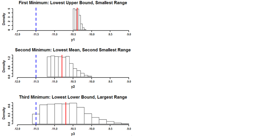
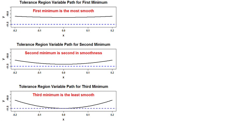
Figure 5. Optimum Selection Measures: The right column has the histograms of the distributions of function values in the tolerance region for three two dimensional concave symmetric local minima. The first minimum has the least range and lowest upper bound. The second has the lowest mean value (vertical red solid line). The third has the lowest lower bound (the blue dashed vertical line, denoting the global minimum). The four measures for quantifying the utility of a minimum are the lower bound, the mean, the upper bound, and the range. The right column of the figure has the variable paths of each of the minima in the tolerance region. They are made by holding one variable constant while varying the other. They show that the smoothness of the minimum is related to the range. The variable paths are relatively flat since the y range has been compressed. If both axes had the same scale, the variable paths would have much more variation along the y axis. The horizontal blue dashed lines are the lower bound of the third minimum for reference.
values for each attribute, we could just concern ourselves with a utility function that is a vector inner product
 , where
  are the weights attached to each attribute by the user and
  are the scaled versions of the attributes for a given optimum as described below. Since the
 are unknowns associated with a probability distribution function, the Bayesian decision approach employs an expected value for determining the utility:
 . The optimum with the maximum expected value (highest utility) is the “best” optimum. The utility values,
 ![]() , of all of the optima rank their utility relative to each other.
, of all of the optima rank their utility relative to each other.
To fill in the details of our utility-based approach, let the importance for each measure be given as a set of weights ![]() for
for  with
with . Each minimum has the four measures mentioned: 1) lower bound for the predicted values within the hypercube tolerance region where the minimum is modeled by the emulator; 2) average value of the predicted values; 3) upper bound for the predicted values; 4) range for the predicted values. It is desirable to scale these predicted values to obtain the values
  where
where
 ,
,  indexes the minima and
  is the number of minima. Scaling is done both to make all attributes have comparable values, as well as to move to a maximum utility framework by flipping the axis so that more desirable values are larger (lower function output values have higher utility). First, a base value,
  , is selected to be a meaningful threshold value for the user, such that any minimum of interest would be smaller than
 . One choice for
  could be the average value of all training points or the average value of the predicted values for a large random sample covering the whole input space. Let
 ![]() be the global minimum value. Let the values for the first three un-scaled attributes, not including the range, be given as
be the global minimum value. Let the values for the first three un-scaled attributes, not including the range, be given as . The scaled values become:

So as to avoid confusion with regard to the lower bound and upper bound some comments are needed. The lower bound unscaled attributes of the minimum,  , become the upper bound attributes,
  , of the scaled measure. The upper bound unscaled attributes,
  , become the lower bound scaled attributes,
 .
.
In other words, the minimum measures are inverted so that they are presented as maximum measures. All scaled values are between 0% and 100%. The range attributes are given by  where
where  refers to the scaled lower bound and
  refers to the scaled upper bound. This scaling of the range yields higher values for smaller ranges which are preferred, and it restricts the range values to an upper limit of 100%.
Because the true  are unknown (unless we happen to have sampled the exact point), we instead use samples,
  , from the emulator’s posterior predictive distribution. As the utility function is similarly based on unknown quantities, we maximize the expected utility [17], where the expectation is taken with respect to the posterior predictive distribution. In practice, we use a Monte Carlo approximation to the expectation, taking an empirical average of sampled iterates from the posterior distribution:
 where
where  indexes the iterates making up the distribution of the
 . Thus the optimal decision is
 ![]() where
where .
.
One further comment concerns the tolerance distance of the hypercube. By default, this is set to one fourth the smallest correlation distance of the emulator model. This distance represents the distance between input points that have significant correlation to each other along a given variable’s axis. The minimum point is correlated to all points within this distance along a given variable’s axis. Other variables have correlation distances greater than or equal this distance. So the minimum point is highly correlated with all points within this distance. Beyond this region, the simulator function may be less reliable.
4. First Illustrative Example
The three minima shown in the explanation of attributes in Section 3, Figure 5, are now used to illustrate the Bayesian decision approach. These three minima are considered to be hypothetically within the input space of a simulator function, having been found by a search for multiple minima. They have the same size tolerance region. A set of training points is selected using a Soboĺ sequence to get well spaced points within each minimum’s hypercube. Using these points, the TGP emulator [18] provides a statistical model of the function within the hypercube region and predicts a large random sample of input points. The iterates of the predicted points form the basic data from which are obtained: 1) The iterates for the lower bound which are the minima of the predicted point iterates; 2) The iterates for the average value which are the mean values for the predicted point iterates; 3) The iterates for the upper bound which are the maxima for the predicted point iterates.
The value of  for this synthetic case is chosen as −6 which makes for a good illustration. This is a convenient value and does not affect the Bayesian decision process, although, the greater the difference,
 ![]() , is, the lesser the differences in the utility values. However, the ordering of the utility values remains the same. For an actual experiment, the user should choose a meaningful value for
, is, the lesser the differences in the utility values. However, the ordering of the utility values remains the same. For an actual experiment, the user should choose a meaningful value for . The lowest iterate for the lower bound of the global minimum is the
 ![]() value. Using the lower bound, average, and upper bound iterates,
value. Using the lower bound, average, and upper bound iterates,  , along with the values for
  and
and![]() , the scaled values,
, the scaled values,  , can then be computed as well as the range iterates
 . Then the Monte Carlo estimates for the utility values are computed. In this case, each measure is weighted equally. The histograms of the scaled iterates are shown in Figure 6 for the three minima.
Notice that the first minimum has the highest scaled lower bound iterates which is expected since it had the lowest upper bound un-scaled y values. The second minimum has the highest scaled average iterates since it had the lowest average un-scaled y values. The third minimum has the highest scaled upper bound iterates since it is the global minimum. Notice too, that the scaled range iterates show that the first minimum has the best range, the second minimum has the second best range, and the third minimum has the worst range (in terms utility contribution). Applying the Bayesian decision approach to find the utility values gives the summary of the utilities shown for each minimum in Figure 7. The mean scaled lower bounds are the black “|”s. The mean scaled averages are the blue “|”s. The mean scaled upper bounds are the red “|”s. There is a horizontal line
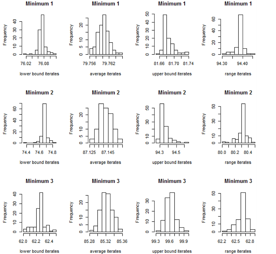
Figure 6. Scaled Iterates for the Three Minima: For each histogram, the x-axis is the emulator predicted value for the iterates. The y-axis is the frequency. The four histograms in each row correspond to a minimum. The columns from left to right are the histograms for the lower bound iterates, the mean scaled iterates, the upper bound iterates, and the range iterates. The first minimum has the highest scaled lower bound iterates, the second minimum has the highest scaled mean iterates, the third minimum has the highest scaled upper bound iterates, and the first minimum has the highest scaled range iterates signifying a smaller range.
joining the scaled measures. The utility values computed from the iterates for the first and third minima are the blue “X”s and the one red “X” is the maximum utility value for the second minimum.
Although, the second optimum (minimum) is selected for equal weights, a different choice for the weights could result in a different optimum selection. For a user who would like a balanced choice that weights all four measures the same, the choice of the second minimum is a reasonable choice.
The user might second guess his/her assignments of the weights and how it affects the utility values. The graph in Figure 7 can be used as a check since it shows the means of three of the four measures for each minimum on a common scale. The range can be inferred from the distance between the lower and upper bound means. In view of the graph, a user who would like less uncertainty regarding the value might be inclined to go with first minimum. Since the graph either confirms or gives the user second thoughts about his/her choices concerning the weights, in the examples that follow, this graph accompanies the tables with the minima data.
5. Second Illustrative Example
In this example, the utility function is applied to the minima for a modified Schubert test function given in
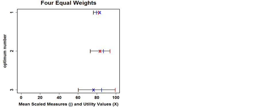
Figure 7. Minima mean scaled measures and utility values for equal weights for three minima (labeled by the y-axis ordinate). The mean scaled lower bounds are black “|”s, the mean scaled averages are blue “|”s, and mean scaled upper bounds are red “|”s. The “X”s are the utility values for the minima.
Equation (5.1) below:
 (5.1)
(5.1)
where  for
for  and
and  is the indicator function equal to one when its argument is true and zero otherwise.
There are several differences from the original Schubert function [19]. The variables are restricted to the interval , rather htan the original
 . In the sums, the cosine terms are multiplied by 0.9 and a displacement of 0.25 is added to the variables in the argument of the cosines. This moves the minima to the interior of the input space. The exponential term multiplying the product of the cosine terms weights the center magnitudes more than the edges, so the dominant minima are in the center of the input space. The two exponential terms added modify the shape and values of the two dominant minima. The one minimum at about (1.2, 0.68) is increased in value and made spikier. The other is increased in value by a little less but smoothed.
A perspective plot of the test function is shown in Figure 8, left, with the minima being peaks to improve visibility. The true minima are listed to the right with coordinates (to two decimal places) and optimal values.
Application of the Algorithm
The algorithm developed in Section 2 was used to search for the minima of the test function. One hundred training points were evaluated for the initial emulator model. The algorithm’s base value parameter  was set to the mean value of the emulator model in the input space, and the level parameter
  was set to 0.8 in order to set the search limit
  high enough to find all eight minima of the function. The algorithm guided the search by passing selected minimum predicted points in the search region to pattern search which then located the minima. Additional points were adaptively sampled to improve the emulator model before each search. After a minimum was located and evaluated by pattern search, additional training points were added to the minimum’s tolerance region (a square centered at the minimum with sides of 0.04 units) in order that the emulator could more accurately model that region. Modeling the tolerance region of each minimum included saving the iterates of the predicted points of a Latin hypercube sample (LHS) covering the tolerance region. At the end of the minima search, the utility function for optimum selection estimated the utility for each minimum from the iterate data saved for each minimum. The eight minima and their utility values are in Table1
In the table, the values for the  and
and ![]() variables are the locations. The value
variables are the locations. The value ![]() is the optimal value,
is the optimal value,  is the mean value of the function’s statistical model in the square (0.04 in width) centered at the
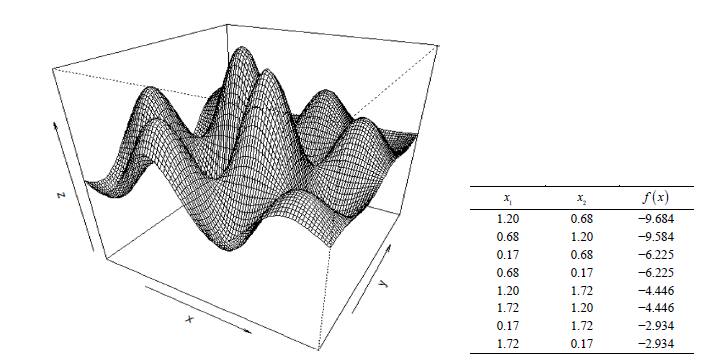
Figure 8. Modified Schubert Test Function: The left panel is a perspective plot of the negative of the modified Schubert function given in Equation (5.1). The negative shows the minima as peaks for better visualization. Both variables have domains [0,2]. The eight minima are listed in the table on the right.
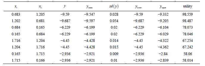
Table 1. The eight minima of the modified Schubert function, ordered by utility value. The input space locations are ![]() and
and![]() ,
,  is the minimum value found by pattern search.
  is the mean value ,
  is the standard deviation,
  is the lower bound, and
  is the upper bound, all in the tolerance region of that minimum. The utility value uses weights which emphasize smoothness or range, (.2,.2,.2,.4), estimating a higher utility for the second smallest minimum that is more smooth than the smallest minimum.
minimum,  is the standard deviation within the square,
  is the lower bound for the
 ![]() values in the square,
values in the square,  is the upper bound. The minimum with the slightly higher optimal value has the highest utility. This is because this minimum is smoother than the global minimum. The weight for range was set higher to favor a smoother minimum. This is where the value of the weight selection by the user is important. For a user that wishes to emphasize optimal value, a greater weight could be given to the upper bound.
The graph showing the means of the lower bound, mean, and upper bound measures along with the utility values is in Figure 9. This appears to be a good choice for an optima with more weight given to the range.
6. Groundwater Remediation Application
We demonstrate our methodology using a computer experiment, the Pump-and-Treat problem described in [20] which involves a groundwater contamination scenario based on the Lockwood Solvent Groundwater Plume Sites located near Billings, Montana. Two plumes (A and B) developed containing chlorinated solvents because of industrial practices near the Yellowstone River. The remediation to prevent contamination of the Yellowstone River involved drilling two pump-and-treat wells in Plume A and four pump-and-treat wells in Plume B. This
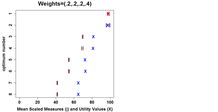
Figure 9. Minima Mean Scaled Measures and Utility Values for Weights = (.2,.2,.2,.4): The x-axis is scaled from 0 to 100% where a higher value indicates more utility. The y-axis has the minimum values on ordinates 1 through 8. The mean scaled lower bounds are black “|”s, the mean scaled averages are blue “|”s, and mean scaled upper bounds are red “|”s. The “X”s are the utility values for the minima (optima). The first minimum has the highest utility value shown as a red “X”. Other weights would give other utility values.
problem has been modeled using a computer simulator where the inputs are pumping rates and pump locations, and the output is the cost. If a given input of these eighteen variables causes contamination of the river, a cost penalty is assessed, so that a minimum cost can be found subject to the constraint of fully preventing contamination of the river. The Lockwood plume site region is about 2 kilometers by 2 kilometers. Plume A is in the lower left part of the region where two pumps are installed. Plume B is more centrally located in the upper part of the region where 4 pumps are installed. An illustration of this site is in Figure 2 of [20].
6.1. Algorithmic Changes for Irregular Simulator Functions
The algorithm discussed in the previous illustration was used in this computer experiment to find multiple minima. However, some simulator functions, even though deterministic, may be very irregular and have many discontinuities. This is true of the simulator function used in the Lockwood Pump-and-Treat problem. The cost is the sum of the pumping rates with a cost penalty added if the location and/or pumping rates of the six pumps cause contamination to occur. There appear to be a very large number of local minima based on a preliminary study, and the contamination penalty creates irregularities in the response surface. These irregularities make it difficult to obtain an accurate emulator model of the underlying function. What this means, in terms of the minima search algorithm discussed herein, is that adjusting the search region based on the computation of the search limit,  , is not viable. Significant minima may be found by searching from any input point free of contamination. The search, however, can be based on starting from a minimum predicted point free of contamination in a search region excluding previous known minima.
To extend the algorithm for irregular functions, the adjustment of the search region distance is bypassed and the control parameter “ratio” (r) which sets the level for minima found is not used. Further, the predicted point with the value  may not be free of contamination. The algorithm attempts to adjust its pumping rates and pump locations to make it free of contamination. If this cannot be done, the algorithm tries the next predicted point with the next lowest value in the search region. This procedure continues until a point free of contamination, or one that can be adjusted to be free of contamination, is found in the search region. This point becomes the starting point for the next search. The search is not ended after two or more duplicate minima are found since, there are so many minima, duplicate minima are not expected. The search can be ended after a given number of minima have been found and at least one is as good as or better than prior information concerning the optimal minimum. If no prior information exists, it is ended after a certain number of minima are found.
Another difference in the approach for irregular functions is that the search region can be made larger. This means the fraction of the maximum distance from known minima to the furthest predicted point can be set smaller so that more predicted points closer to known minima are included in the region as possible starting points for the next search. The reasoning here is that any input point free of contamination could lead to a promising minimum if used as a starting search point. This can be true even if it is near a known minimum.
The starting step size for pattern search is determined in the same way. Here, though, optimization runs show that the starting points in the Pump-and-Treat problem are often far enough from known minima in the input space that the initial step size does not need modification. This has been true even after many minima have been found. There is one other consideration regarding initial step size: It should be less than the cost penalty for contamination. The reasoning here is that, if a reduction in the pumping rate exceeds this cost penalty, pattern search could step to a point with contamination since it would have a lesser cost than a previous contamination free point. For the optimization methods herein, the cost penalty is chosen small enough so that the TGP emulator can follow the irregular simulator function, since a large discontinuous jump in the cost can present a problem for the emulator (TGP can handle axis-aligned discontinuities, but must work harder when discontinuities are not axis-aligned).
6.2. Application of the Algorithm
The optimization was run to find eight minima. The training points were provided by a global sensitivity analysis based on points randomly sampled within the plumes. The algorithm guided the minimum search by selecting starting points free of contamination from search regions distanced from known minima to send to pattern search. Before each search (after the first search), the point with the highest standard deviation and the point with maximum expected improvement were added to the training point set to improve the emulator model. For each minimum found, the pump locations of the minimum found were “centered”, as we found that if the pump location were moved slightly from its minimum location, contamination could occur. By testing locations around the minimum locations, the pump could be relocated so it was within a contamination free zone, that is, movements of ±0.5 ft in any direction would not result in contamination. Also, it was found that increasing pumping rates, once the pumps were centered, did not cause contamination. Therefore, the tolerance region for pump location is the pump centered location ±0.5 ft and the tolerance region for pumping rate is , where
  is the minimum pumping rate of pump
![]() . This tolerance region is based on the feasibility of of locating pumps within ±0.5 ft and controlling pumping rates within
. This tolerance region is based on the feasibility of of locating pumps within ±0.5 ft and controlling pumping rates within![]() . Within this tolerance region, the pumping system remains contamination free. For each minimum found, the emulator modeled the tolerance region of the minimum with the aid of additional points sampled from that region. Then the emulator used this model to predict the points of a LHS covering the region (or other random sample with good spatial coverage) along with all their iterates. These are then saved for the estimation of the utility values after the search for the minima has ended. For this application, all four measures were given equal weights.
. Within this tolerance region, the pumping system remains contamination free. For each minimum found, the emulator modeled the tolerance region of the minimum with the aid of additional points sampled from that region. Then the emulator used this model to predict the points of a LHS covering the region (or other random sample with good spatial coverage) along with all their iterates. These are then saved for the estimation of the utility values after the search for the minima has ended. For this application, all four measures were given equal weights.
The table on the left of Figure 10 has the eight minima found by our optimization method.  is the minimum cost value for the input of six rates and locations.
  is the mean cost value,
  is the standard deviation of the
  values,
  is the lower bound,
  is the upper bound, all within each tolerance region. “Utility” is the utility value computed from the
  iterates in the tolerance region. All values have been rounded to the nearest integer except for the standard deviations and the utility values which are rounded to one decimal place. In the table, the minima are ordered by utility value.
Figure 10 shows the means of the lower bound, mean, and upper bound measures along with the utility values. This appears to be a good choice for equal weights.
7. Conclusion
We propose a search algorithm for efficiently exploring the whole input space, and a utility function for optimum selection that makes use of Bayesian decision theory. It quantizes the attributes of interest in optimum selection, the optimum’s smoothness and value, and takes into account the user’s specific needs. The four measures used to quantize the attributes of interest are obtained from the predictions of a statistical emulator model in the tolerance region. Since this emulator covers a small region relative to the input space it can be made accurate with a small number of training points. In other words, it makes efficient use of function evaluations. While it works best in combination with an online search algorithm, the selection methodology can also be employed on a pre-existing set of function evaluations.

Figure 10. The eight Lockwood problem minima found by our optimization method are shown in the table on the left, where  is the minimum cost value,
  is the mean cost value,
  is the standard deviation of the cost,
  is the lower bound of the cost, and
  is the upper bound of the cost, all within each tolerance region. The plot on the right shows the scaled measures and utility for these minima. The mean scaled lower bounds are black “|”s, the mean scaled averages are blue “|”s, and mean scaled upper bounds are red “|”s. The “X”s are the utility values for the minima (optima). The first minimum has the highest utility value shown as a red “X”.
Acknowledgements
Partial funding was provided by Sandia National Laboratories and by NSF grant DMS 0906720.
REFERENCES
- K. C. Tan, E. F. Khor and T. H. Lee, “Multiobjective Evolutionary Algorithms and Applications,” Springer, Berlin, 2005.
- E. Zitler and L. Thiele, “Multiobjective Evolutionary Algorithms: A Comparative Case Study,” IEEE Transactions on Evolutionary Computation, Vol. 3, No. 4 1999, pp. 257-271. http://dx.doi.org/10.1109/4235.797969
- D. E. Goldberg, “Genetic Algorithms in Search, Optimization, and Machine Learning,” Addison Wesley, 1989.
- J. H. Holland, “Adaption in Natural and Artificial Systems,” University of Michigan Press, Ann Arbor, 1975.
- J. H. Holland, “Genetic Algorithms and the Optimal Allocation of Trials,” SIAM Journal on Computing, Vol. 2, No. 2, 1975, pp. 88-105.
- J. Kennedy and R. C. Eberhart, “Particle Swarm Optimization,” IEEE International Conference on Neural Networks, Piscataway, 1995.
- T. Santner, B. Williams and W. Notz, “The Design and Analysis of Computer Experiments,” Springer, Berlin, 2003. http://dx.doi.org/10.1007/978-1-4757-3799-8
- R. Gramacy and H. Lee, “Bayesian Treed Gaussian Process Models with Application to Computer Modeling,” Journal of the American Statistical Association, Vol. 103, No. 483, 2008, pp. 1119-1130. http://dx.doi.org/10.1198/016214508000000689
- A. Gelman, J. B. Carlin, H. S. Stern and D. B. Rubin, “Bayesian Data Analysis,” Chapman & Hall, London, 2004.
- M. Taddy, H. Lee, G. Gray and J. Griffin, “Bayesian Guided Pattern Search for Robust Local Optimization,” Technometrics, Vol. 51, No. 4, 2009, pp. 389-401. http://dx.doi.org/10.1198/TECH.2009.08007
- L. Bastos and A. O’Hagan, “Diagnostics for Gaussian Process Emulators,” Technometrics, Vol. 51, No. 4, 2009, pp. 425-438. http://dx.doi.org/10.1198/TECH.2009.08019
- H. Lee, R. Gramacy, C. Linkletter and G. Gray, “Optimization Subject to Hidden Constraints via Statistical Emulation,” Pacific Journal of Optimization, Vol. 7, No. 3, 2011, pp. 467-478.
- D. Jones, M. Shonlau and W. Welch, “Efficient Global Optimization of Expensive Blackbox Functions,” Journal of Global Optimization, Vol. 13, No. 4, 1998, pp. 455-492. http://dx.doi.org/10.1023/A:1008306431147
- G. A. Gray and T. G. Kolda, “Algorithm 856: APPSPACK 4.0: Asynchronous Parallel Pattern Search for Derivative-Free Optimization,” ACM Transactions on Mathematical Software, Vol. 32, No. 3, 2006, pp. 485-507.
- S. M. Wild and C. A. Shoemaker, “Global Convergence of Radial Basis Function Trust Region Algorithms for Derivative-Free Optimization,” SIAM Review, Vol. 55, No. 2, 2013, pp. 349-371. http://dx.doi.org/10.1137/120902434
- J. Berger, “Statistical Decision Theory and Bayesian Analysis,” Springer-Verlag, Berlin, 1985. http://dx.doi.org/10.1007/978-1-4757-4286-2
- M. H. DeGroot, “Optimal Statistical Decisions,” Wiley, New York, 2004. http://dx.doi.org/10.1002/0471729000
- R. B. Gramacy, “Tgp: An R Package for Bayesian Nonstationary, Semiparametric Nonlinear Regression and Design by Treed Gaussian Process Models,” Journal of Statistical Software, Vol. 19, No. 9, 2007, pp. 1-48.
- A.-R. Hedar and M. Fukushima, “Tabu Search Directed by Direct Search Methods for Nonlinear Global Optimization,” European Journal of Operational Research, Vol. 127, No. 2, 2006, pp. 329-349. http://dx.doi.org/10.1016/j.ejor.2004.05.033
- L. S. Matott, K. Leung and J. Sim, “Application of Matlab and Python Optimizers to Two Case-Studies Involving Groundwater and Contaminant Transport Modeling,” Geospatial Cyberinfrastructure for Polar Research, Vol. 37, No. 11, 2011, pp. 1894- 1899.
Appendix
Pseudo Code for Optimization
Initialize parameters:
Evaluate an LHS of training points Set base value  and level parameter
Set loop count  to 0 Set tolerance region width or define tolerance region parameters Set interval width
Begin loop for minimum search:
Increment 
Model simulator function with emulator and current training points and predict a large random sample (LHS) of points Determine minimum predicted point  and value
If 
Construct array with predicted points, their minimum distance from the nearest minimum and compute search region distance
![]() from maximum predicted point distance
from maximum predicted point distance :
: 
Order array by decreasing distance for computational efficiency Determine , distance from
  to the nearest minimum Endif Begin case processing:
Case 1: If  is 1Start pattern search from
  to find first minimum with location
  and value
Set lowest minimum,  , to
, to 
Set search limit, 
Case 2: If  and
and  and the distance interval,
  , has all predicted point values
 Start pattern search from
  to find the next minimum with location
  and value
If , reset
  to
to 
Case 3: If  and
and  and distance interval,
  , has predicted point values
 Increase search region distance from known minima by increments until Case 2 or Case 4 occurs and proceed to Case 2 or Case 4 Case 4: If
  and
and Start pattern search from
  to find the next minimum with location
  and value
If , reset
  to
to 
Case 5: If  and
and Decrease search region distance from known minima by increments until Case 4 occurs and proceed to Case 4 End case processing If duplicate minimum found, quit minimum search loop Adaptively sample points for model improvement Model tolerance region for current minimum and save predicted point iterates for the utility function for optimum selection End loop for minimum search Invoke utility function for optimum selection to estimate utility values
End Pseudo Code for Optimization