Applied Mathematics
Vol.4 No.8A(2013), Article ID:35178,18 pages DOI:10.4236/am.2013.48A009
Mathematical Rotordynamic Model Regarding Excitation Due to Elliptical Shaft Journals in Electrical Motors Considering the Gyroscopic Effect
Siemens AG, Industry, Drive Technologies, Large Drives, Products, Research & Development, Nuremberg, Germany
Email: werner.ulrich@siemens.com
Copyright © 2013 Ulrich Werner. This is an open access article distributed under the Creative Commons Attribution License, which permits unrestricted use, distribution, and reproduction in any medium, provided the original work is properly cited.
Received April 24, 2013; revised May 24, 2013; accepted June 1, 2013
Keywords: Rotordynamics; Elliptical Shaft Journals; Orbit; Vibrations
ABSTRACT
The paper presents a mathematical rotordynamic model regarding excitation due to elliptical shaft journals in sleeve bearings of electrical motors also considering the gyroscopic effect. For this kind of excitation, a mathematical rotordynamic model was developed considering the influence of the oil film stiffness and damping of the sleeve bearings, the stiffness of the end-shields and bearing housings, the stiffness of the rotor, the electromagnetic stiffness in the air gap of the electrical motor and the mass moment of inertia of the rotor and therefore also considering the gyroscopic effect. The solution of the linear differential equation system leads to the mathematical description of the absolute orbits of the shaft centre, the shaft journals and the bearing housings and to the relative orbits between the shaft journals and the bearing housings. Additionally, the bearing housing velocities can also be derived with this mathematical rotordynamic model.
1. Introduction
In electrical motors many different kinds of excitation exist, like mechanical unbalance, misalignment of the coupling [1-3] and electromagnetic forces—e.g. unbalanced magnetic pull [4-11]—which may cause vibrations. In this paper a special kind of excitation caused by elliptical shaft journals [12], in conjunction with sleeve bearings [13-17], is investigated, also considering the gyroscopic effect of the rotor. Due to the machining process of the rotor, the shaft journals may get a marginal form deviation, so that they are no longer cylindrical. In some cases the shaft journals may become an elliptical shape instead of circular shape. However, the form deviation D is usually very small, about 0.0005% - 0.002% referred to the diameter of the shaft journal. In standards and specifications the so called run out of the shaft journals is limited by e.g. the standard IEC 60034-14 [18] and the standard API 541 [19]. Due to this form deviation the centre of the shaft journal V changes its position in the sleeve bearings as the rotor rotates, leading to a dynamic displacement on the oil film (Figure 1). This dynamic displacement of the shaft journals on the oil film of the sleeve bearing represents an excitation for the rotor dy-
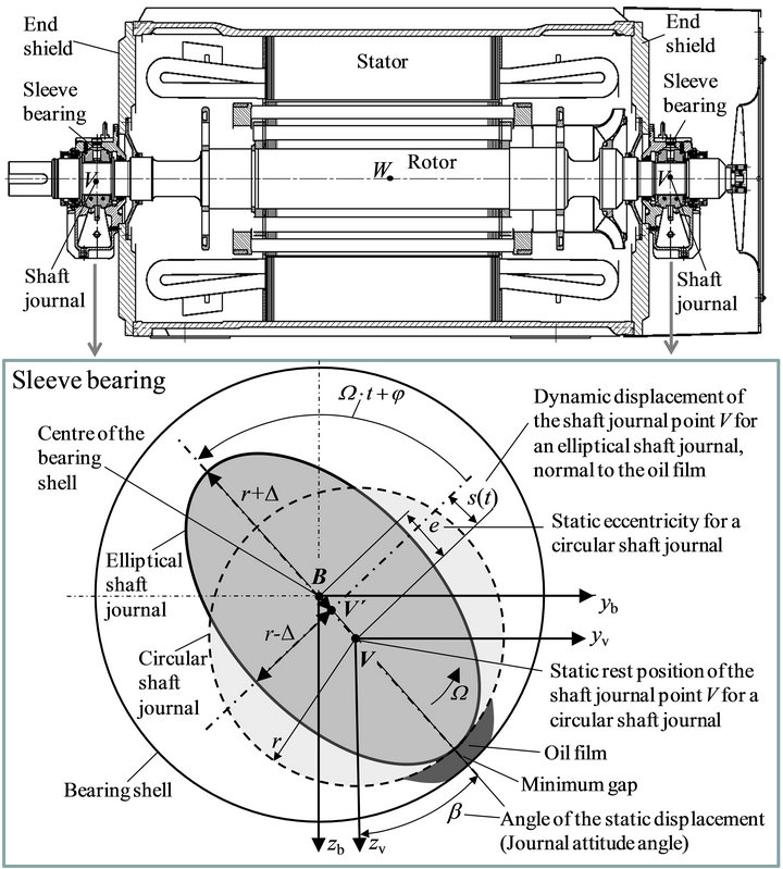
Figure 1. Two-pole induction motor with flexible shaft and elliptical shaft journals in sleeve bearings.
namic system, leading to forced vibrations. This was derived in [12], but only with a simplified rotordynamic model without considering the mass moments of inertia of the rotor and the gyroscopic effect.
The developed rotordynamic model in [12] is more suitable for a stiff rotor design, where only the first bending mode—“V-shape”—of the rotor is of interest. For this mode, the influence of the inertias of the mass moments and the gyroscopic effect is usually small for electrical rotors. For flexible rotors (Figure 1) also higher bending modes, like “S-shape”, have to be considered, because here the natural frequencies of these modes are much lower as for a stiff rotor design and may be excited by the dynamic displacement of elliptical shaft journals.
Therefore the presented rotordynamic model here is an enhancement of the model presented in [12], additionally considering mass moments of inertia of the rotor and the gyroscopic effect. So, the here presented rotordynamic model is also suitable for flexible rotors.
2. Rotordynamic Model
The rotordynamic model is described in Figure 2, where the rotor rotates with the rotor angular frequency W. The rotordynamic model represents an enhancement of the rotordynamic model shown in [12], where the rotor mass was concentrated as a lumped mass, without mass moments of inertia and therefore without considering the gyroscopic effect. The enhancement of the here presented rotordynamic model in Figure 2 is, that the rotor mass has now also mass moments of inertia, so that also the gyroscopic influence can be considered.
The rotordynamic model contains the rotor mass m, which is concentrated as a lumped mass on an elastic shaft in the point W, with the mass moment of inertia Θp at the rotational axis and the mass moment of inertia Θa, normal to the rotational axis. The point W is positioned in the centre of the rotor shaft and with distance of l1 and l2 to the sleeve bearings—bearing (1) and bearing (2), considering a non-symmetrical position. The oil film stiffness and damping of the sleeve bearings are described by the oil film stiffness matrices Cv1 and Cv2 and the oil film damping matrices Dv1 and Dv2. In the oil film stiffness and damping matrices the oil film coefficients cij and dij are included, which can be derived by solving the Reynolds differential equation [13-17]. The stiffness matrices Cb1 and Cb2 describe a series connection of the stiffness of the sleeve bearing housings, the end shields and the stator housing in the area of the end shields. Usually, the damping of the bearing housing, end-shield and stator housing is so low, that it can be neglected. In this model, the machine foundation is assumed to be rigid, simulating a massive foundation [18,19].
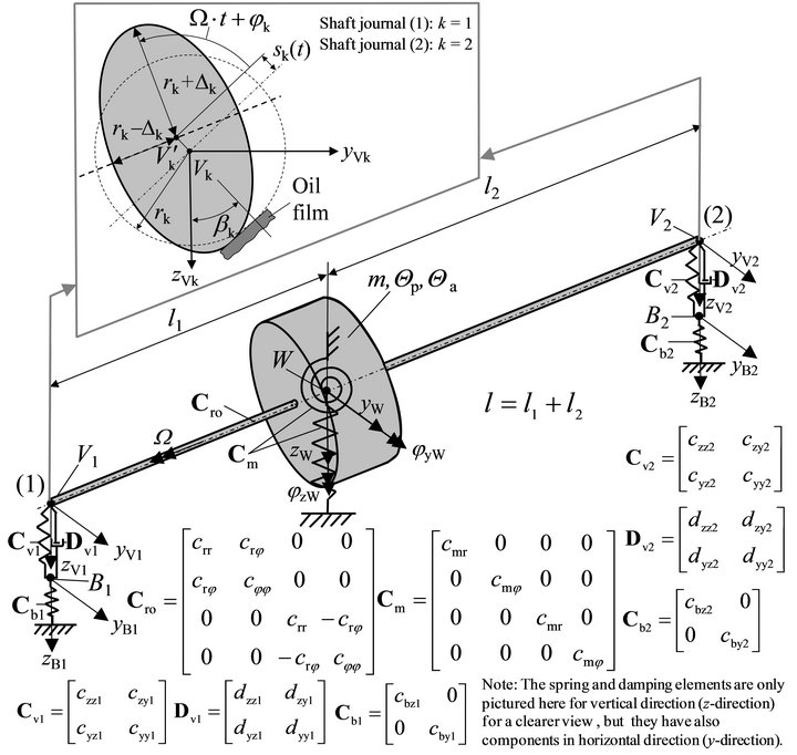
Figure 2. Rotordynamic model.
The stiffness of the rotor is described in the stiffness matrix Cro, where crr is the radial stiffness, cjj the angular stiffness and crj the cross-coupling stiffness of the rotor itself in point W, when the rotor is supported in rigid bearings. Here, the cross-coupling stiffness crj means that a radial force at the shaft centre point W also causes an angular displacement of the shaft centre point W. However, a moment at the shaft centre point W also causes a translational displacement of the shaft centre point W. In the model described in [12], only a radial stiffness was considered. The derivation of the rotor stiffness matrix is based on [3,11].
For electrical machines, there is an electromagnetic coupling between the rotor and the stator [4-11], which can be described by the magnetic spring matrix Cm. In addition to the radial magnetic spring constant cmr— which is described in the rotordynamic model in [12]— now also an angular magnetic spring constant cmj is used, which is derived in [11]. The magnetic spring constants cmr and cmj have a negative reaction. This means that a radial displacement of the rotor mass creates an electromagnetic force that tries to magnify the radial displacement. However, an angular displacement of the rotor mass creates an electromagnetic moment which also tries to magnify the angular displacement. Electromagnetic field damping is not considered in the simplified model.
The excitation in this model is only caused by elliptical shaft journals. Other excitations like mechanical unbalance, unbalanced magnetic pull etc. are not considered in this paper, but of course they can be superposed. Therefore, the excitation is only caused by the forced displacement of each elliptical shaft journal on the oil film in each sleeve bearing. Referring to [12], the forced displacement s1(t) and s2(t) of the shaft journal centre point V1 and V2 normal to the oil film, which means in direction of static eccentricity, can be described by:
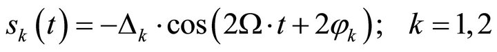 (1)
(1)
In the model five fixed coordinate systems are used. One coordinate system is positioned at the static rest position of the point W. In this coordinate system the translation of the shaft centre point W is described in the coordinates zW and yW and the rotation of W is described in the coordinates jzW and jyW. The translation of the shaft journals V1 and V2 are described in the separate coordinate systems (zV1; yV1) and (zV2; yV2), which are fixed at the static rest positions of the shaft journals. The translation of the bearing housing points B1 and B2 are also described in the separate coordinate systems (zB1; yB1) and (zB2; yB2), which are positioned at the static rest position of the bearing housing points.
3. Mathematical Description
To derive the equations of motion, it is necessary to split up the vibration system into five individual systems:
- Rotor mass system for shaft centre point W;
- Shaft journal systems for shaft journal point V1 and V2;
- Bearing housing systems for bearing housing point B1 and B2.
3.1. Kinematic Constraints
Referring to [11], the kinematic constraints between the radial displacements of the shaft journals V1 and V2 and the radial and angular displacement of the rotor centre point W, for a rigid rotor, are described by (Figure 3):
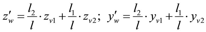 (2)
(2)
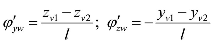 (3)
(3)
3.2. Rotor Mass System
The forces and moments, which act on the shaft centre point W, are shown in Figure 4. A complex coordinate system is introduced to afterwards describe the radial movement of the shaft centre point W with a complex vector rw. The complex vector r¢w describes the radial movement of the shaft centre point W, as if the rotor would be rigid. Therefore, the complex vector rw-w¢ describes the radial elastic deformation of the shaft.
The equilibrium of forces and moments leads to following equations:
 (4)
(4)
 (5)
(5)
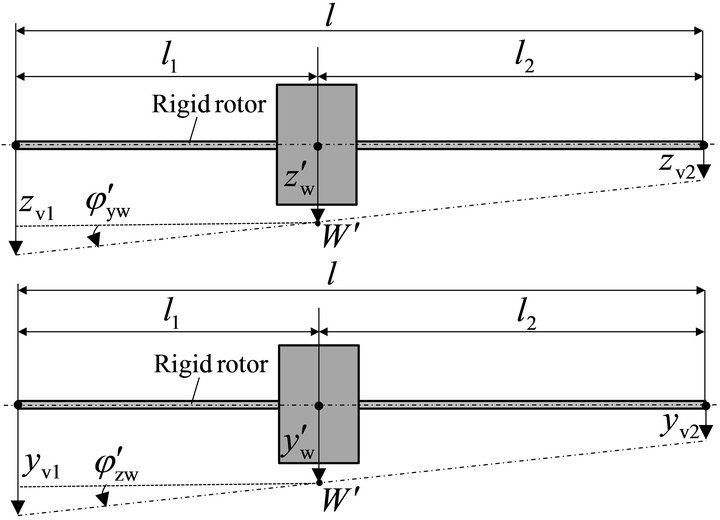
Figure 3. Kinematic constrains.
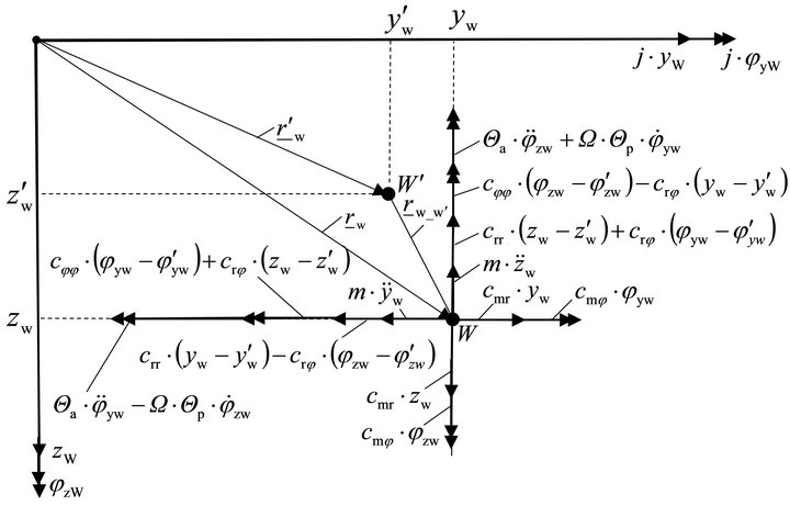
Figure 4. Rotor mass system.
 (6)
(6)
 (7)
(7)
3.3. Shaft Journal System
The forces acting on the shaft journal point V1 are shown in Figure 5. The complex vector rv1 describes the radial movement of the shaft journal point V1, the complex vector rb1 the movement of the bearing housing point B1. The complex vector s1 describes the forced displacement of the shaft journal point V1 on the oil film due to the elliptical shape, as if the rotor would be without mass and electromagnetism. Therefore the complex vector rv1-v1¢ describes the radial displacement of the shaft journal on the oil film, caused by the mass inertias and electromagnetism. F1y and F1z are oil film forces, which correspond to the forced displacement s1.
The equilibrium of forces at shaft journal point V1 lead to following equations:
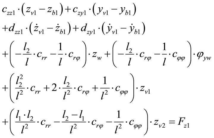 (8)
(8)
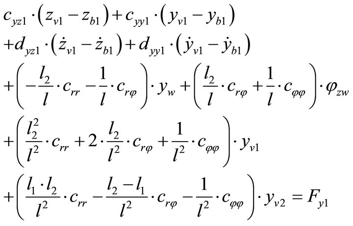 (9)
(9)
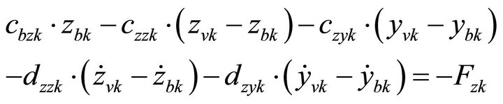
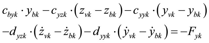
The forces acting on the shaft journal point V2 are shown in Figure 6.
The equilibrium of forces at shaft journal point V2 lead to following equations:
 (10)
(10)
 (11)
(11)
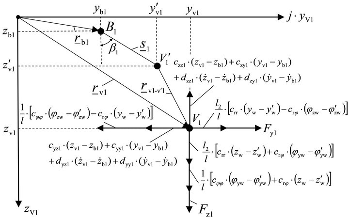
Figure 5. Shaft journal system for shaft journal (1).
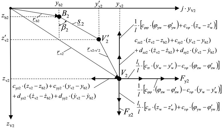
Figure 6. Shaft journal system for shaft journal (2).
Referring to [12], the oil film forces Fzk and Fyk—for bearing (1): k = 1; for bearing (2): k = 2—are:
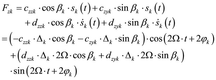 (12)
(12)
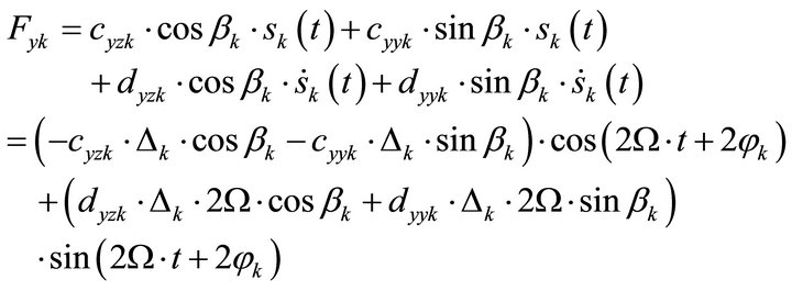 (13)
(13)
3.4. Bearing Housing System
The forces acting on the bearing housing points B1 and B2 are shown in Figure 7.
The equilibrium of forces at the bearing housing points B1 and B2 leads to following equations:
 (14)
(14)
 (15)
(15)
3.5. Differential Equation System
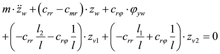
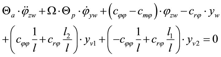
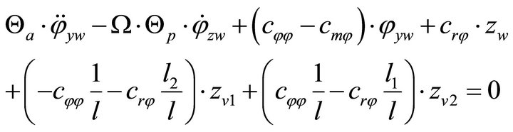
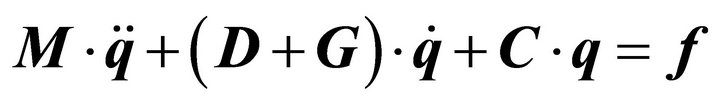
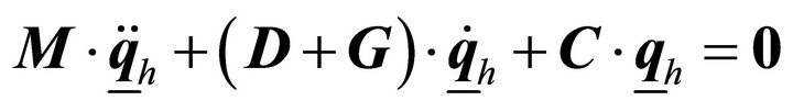
With the Equations (4)-(15), the inhomogeneous differential equation, described by mass matrix M, damping matrix D, gyroscopic matrix G, stiffness matrix C, coordinate vector q, and excitation vector f, can be derived:
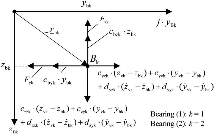
Figure 7. Bearing housing systems.
 (16)
(16)
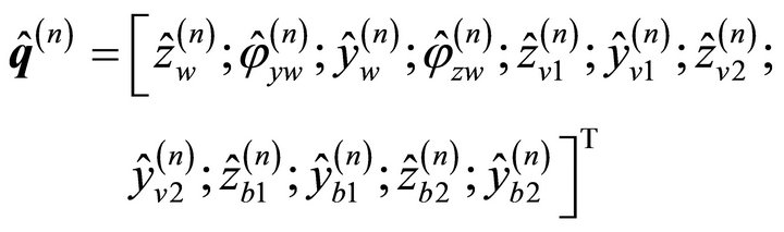
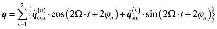
The coordinate vector q is described by:
 (17)
(17)
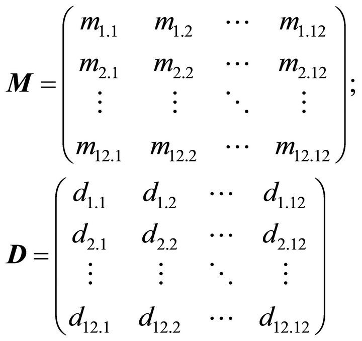
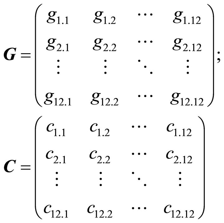
Referring to [11], the mass matrix M, damping matrix D, gyroscopic matrix G, stiffness matrix C are described by:
 (18)
(18)
 (19)
(19)
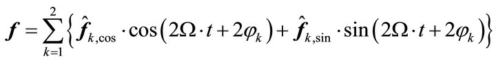
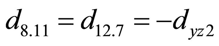
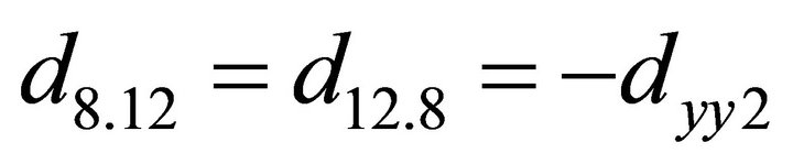
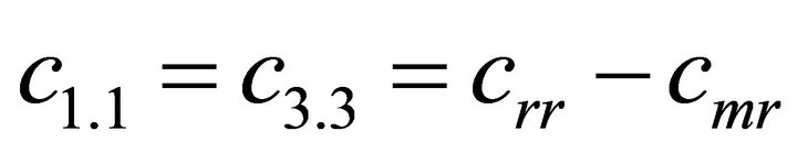
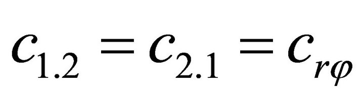
with the matrix coefficients mi.j, di.j, gi.j, ci.j  , described in the Appendix. The excitation vector f is described by:
 (20)
(20)
3.6. Natural Vibrations
The natural vibrations can be calculated by solving the homogeneous differential equation, using a complex formulation, following [3].
 (21)
(21)
With the formulation 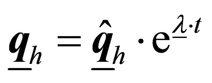 the complex eigenvalues
 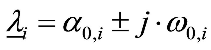 and eigenvectors
  can be calculated well as modal damping D0,i of each eigenmode with [3]:
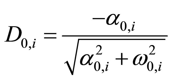 (22)
(22)
For a numerical estimation of the eigenvalues, it is sometimes easier to use the equation of state, where 0 is the zero matrix and I is the unit matrix:
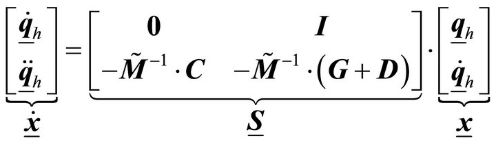 (23)
(23)
But therefore, the mass matrix has to be inverted. This is not possible, using the mass matrix M, because of its singularity with m5.5 = m6.6 = m7.7 = m8.8 = m9.9 = m10.10 = m11.11 = m12.12 = 0.
Therefore, an alternative mass matrix  has to be used, putting a fictitious mass mf (with
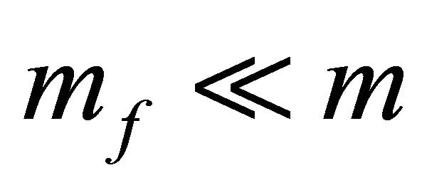 ; e.g. mf » m·10−6) at the nodes Vk and Bk.
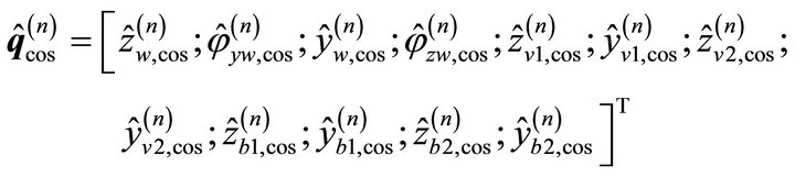
3.7. Forced Vibrations
To derive the forced vibrations, the inhomogeneous differential equation has to be solved. The excitation vector f can be split into sinusoidal and cosine components:
 (24)
(24)
with:
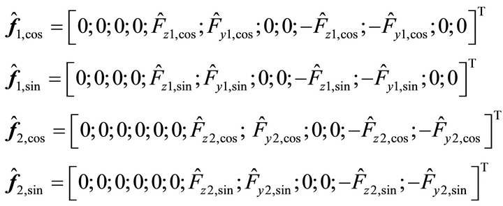 (25)
(25)
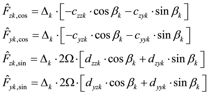 (26)
(26)
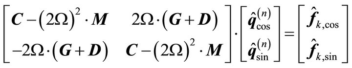
The following formulation is chosen to solve the differential equation:
 (27)
(27)
with: 
 (28)
(28)
 (29)
(29)
 (30)
(30)
The index n describes which shaft journal is causing the excitation. The formulation leads to following matrix formulation:
 (31)
(31)
By solving this matrix equations for each single excitation, the amplitude vectors  and
and  can be computed and the solutions superposed:
 (32)
(32)
3.8. Absolute Orbits
Referring to [12], the complex coordinate systems are now used to describe the orbit movement of each point (W, V1, V2, B1, B2). Index c is used for the complex pointers rc, with:
 with:
with: (33)
(33)
The solutions rc can be described by one complex vector rotating in the direction of rotor rotation (+2W) and one rotating opposite to the direction of rotor rotation (−2W).
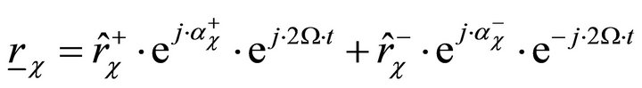 (34)
(34)
with:
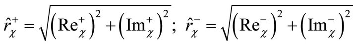 (35)
(35)
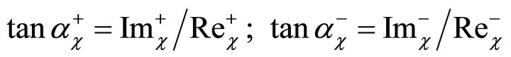 (36)
(36)
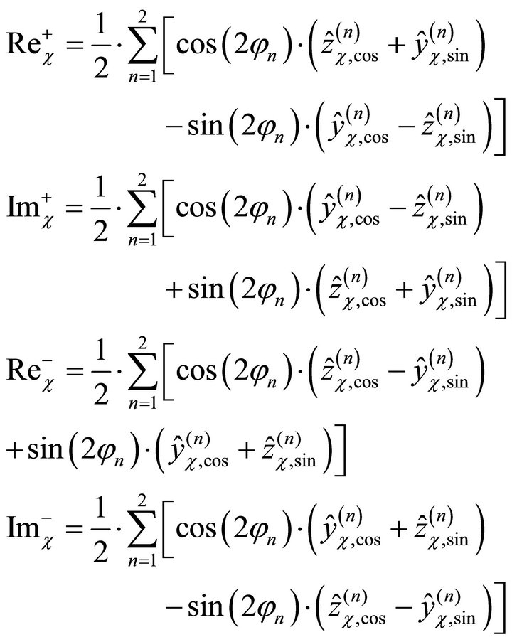 (37)
(37)
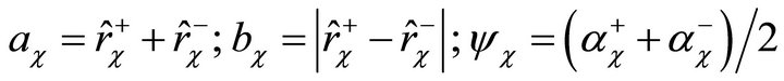
The description of the orbit shape is shown in Figure 8.
The orbit shape of each point (W, V1, V2, B1, B2) can be described by the ellipse parameters with the semi-major axis ac, the semi-minor axis bc and the angle of the major axis yc, referring to [12]:
 (38)
(38)
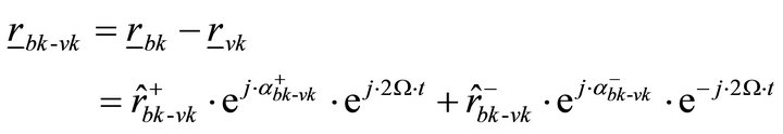
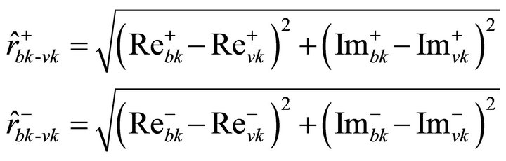
3.9. Relative Orbits
For the evaluation of the vibration quality also the relative orbits between the bearing housing points Bk and the shaft journal points Vk have to be analyzed to identify whether the oil film in the sleeve bearings could be critically disturbed [18,19]. Therefore, vector rbk-vk describes the relative orbit between the shaft journal points Vk and the bearing housing points Bk, referring to [12]:
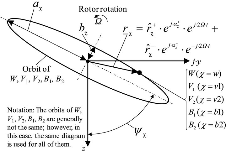
Figure 8. Absolute orbits described by ellipse parameters.
 (39)
(39)
with:
 (40)
(40)
 (41)
(41)
3.10. Bearing Housing Vibrations
In addition to the absolute and relative shaft displacements also the vibration velocities of the bearing housings are used in practice to evaluate the vibration quality of the motor [18,19]. Referring to [12], the bearing housing vibrations can be calculated by:
• Vibration velocity in z-direction:
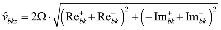 (42)
(42)
• Vibration velocity in y-direction:
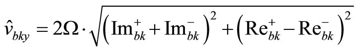 (43)
(43)
4. Numerical Example
In this chapter a two-pole induction motor is analyzed. The motor data are described in Table 1.
The oil film stiffness and damping coefficients for the two bearings are shown in Figures 9 and 10. However, here both sleeve bearings are identical, the oil film stiffness and damping coefficients are different. The reason is that the rotor mass is not symmetrically positioned between the two bearings (l1 ¹ l2).
In Figure 11 the angle b of the static displacement is shown for both bearings.
4.1. Natural Vibrations
Before the forced vibrations due to elliptical shaft journals are analyzed, the natural vibrations are investigated. First, the natural frequencies f0,i and the modal damping values D0,i are calculated depending on the rotor speed (Figure 12).
The modal damping values of mode 1 and mode 2, D01 and D02, are very high (>0.58) in the whole speed range and therefore not pictured in Figure 12. The splitting of the natural frequencies of mode 5 and mode 6 is mainly caused by gyroscopic effect. Due to the excitation with twice the rotor speed (2fr = W/p), three critical speeds occur, where the 2fr line intersects the natural frequencies (Figure 12). The natural mode shapes at the three critical speeds—at the intersection points—are pictured in Figure 13. The gyroscopic effect has the strongest influence on the third critical speed (nc3; mode 5), because the rotor shaft centre point W makes a tumbling motion here.
4.2. Forced Vibrations
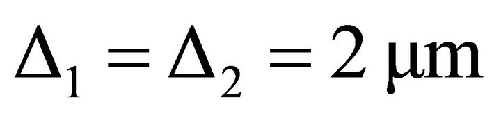
After the natural vibrations and the critical speeds have been calculated, the forced vibrations caused by the elliptical shaft journals are analyzed. Both shaft journals (1) and (2) are assumed to be elliptical with a form deviation of 2 μm, which is a realistic magnitude for this size of the shaft journal:
 (44)
(44)
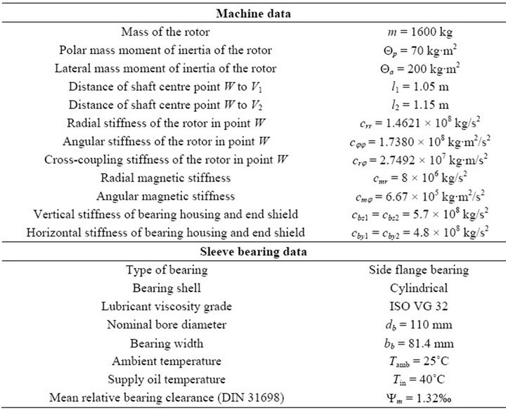
Table 1. Data of the two-pole induction motor.
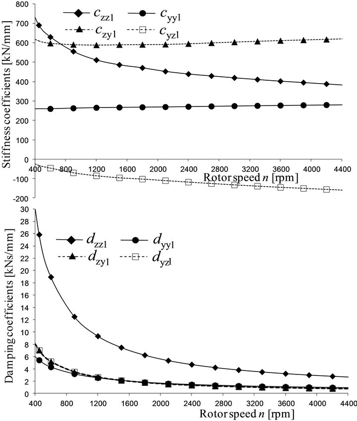
Figure 9. Oil film stiffness and damping coefficients of bearing (1).
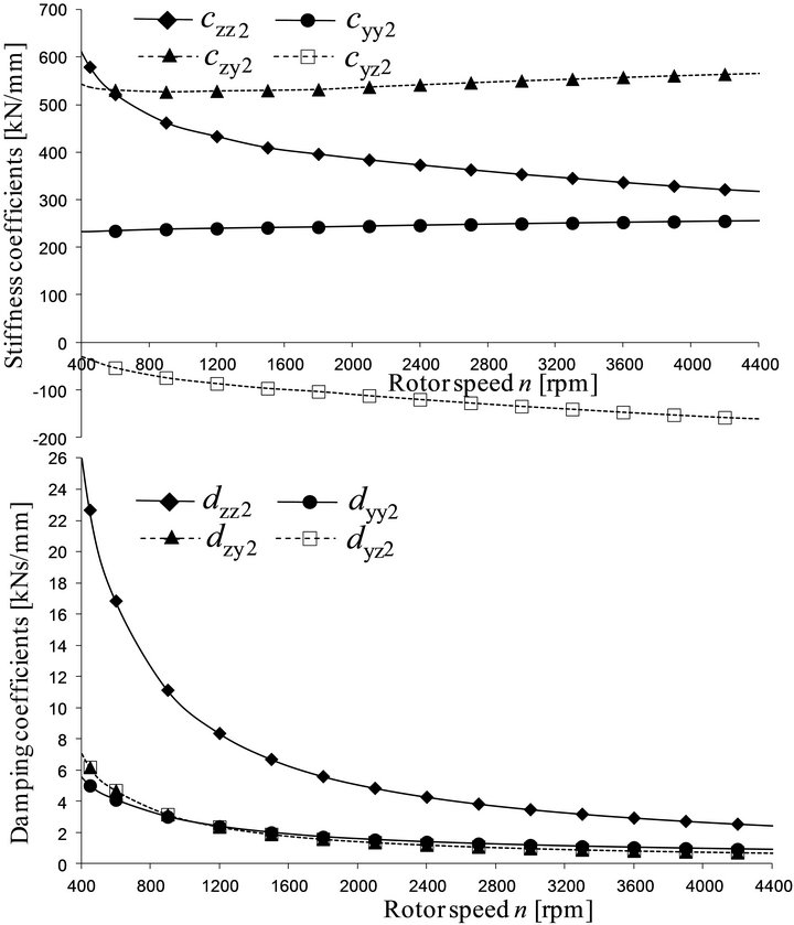
Figure 10. Oil film stiffness and damping coefficients of bearing (2).
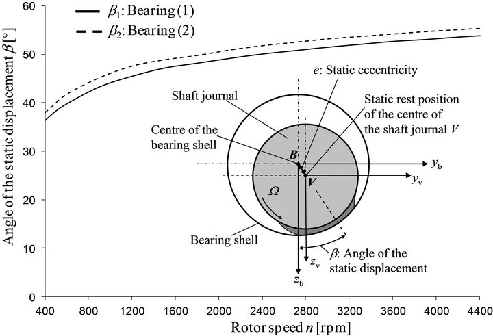
Figure 11. Angle b of the static displacement in the sleeve bearings.
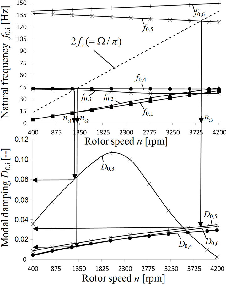
Figure 12. Critical speed map with natural frequencies and modal damping values.
To analyze different phase angels, the angle Dj is introduced as the differential angle, which describes the different orientation of the elliptical shaft journals to each other.
 (45)
(45)
Here, the differential angle Dj is varied between 0˚ and 90˚. Considering different rotor speeds n—from 400 rpm up to 4200 rpm—and the different differential angles Dj—from 0˚ up to 90˚, the semi-major axis of the absolute orbits of the shaft centre point W, the shaft journal points V1 and V2 and the bearing housing points B1 and B2 are calculated as well as the semi-major axis of the relative orbits between the shaft journal points V1 and B1 and V2 and B2. Additionally, the vibration velocities at the bearing housing are calculated.
Semi-major axis of the absolute orbits:
The semi-major axis of the absolute orbits of the shaft centre point W is shown in Figure 14. The maximum value 71.74 μm occurs at a rotor speed of 1293 rpm and at a differential angle of 0˚.
The semi-major axes of the absolute orbits of the shaft journal points V1 and V2 are shown in Figures 15 and 16. Two maxima are obvious in each figure. For shaft journal point V1 (Figure 15) the maxima occur at a rotor speed of 1293 rpm and at a differential angle of 12˚ with a magnitude of 8.58 μm and at a rotor speed of 3782 rpm
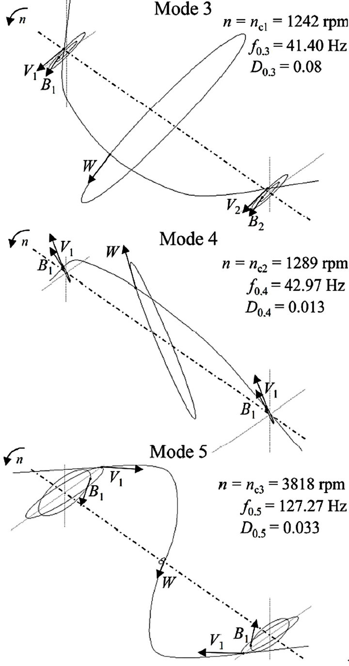
Figure 13. Natural mode shapes at the critical speeds.
and at a differential angle of 90˚ with a magnitude of 5.15 μm. For shaft journal point V2 (Figure 16), the maxima occur at the same speed as for V1, but with different magnitudes and other differential angles. The first maximum occurs at 1293 rpm with a differential angle of 0˚ and a magnitude of 7.93 μm. The second maximum occurs at 3782 rpm with a differential angle of 72˚ and a magnitude of 4.31 μm.
The semi-major axes of the absolute orbits of the bearing housing points B1 and B2 are shown in Figures 17 and 18. Two maxima are obvious in each figure. For B1 (Figure 17) the maxima occur at a rotor speed of 1293 rpm and at a differential angle of 0˚ with a magnitude of 8.34 μm and at a rotor speed of 3820 rpm and at a differential angle of 87˚ with a magnitude of 3.0 μm. For B2 (Figure 18), the maxima occur again at the same speed as for B1. The first maximum occurs at a rotor speed of 1293 rpm with a differential angle of 0˚ and a magnitude of 7.88 μm. The second maximum occurs at a rotor speed of 3820 rpm with a differential angle of 90˚ and a magnitude of 2.21 μm.
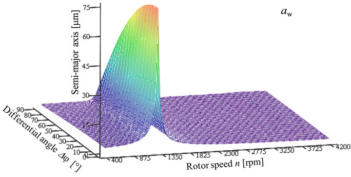
Figure 14. Semi-major axis aw of the absolute orbits of the shaft centre point W.
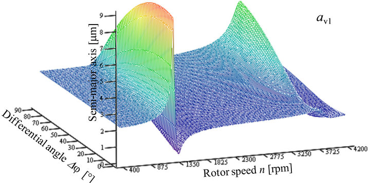
Figure 15. Semi-major axis av1 of the absolute orbits of the shaft journal point V1.
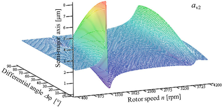
Figure 16. Semi-major axis av2 of the absolute orbits of the shaft journal point V2.
Comparing the maxima of the figures with the critical speeds of Figure 12 it can be shown, that the rotor speeds of the maxima are near to the critical speed nc2 and nc3. The marginal differences are mostly caused by the damping and influenced by the mode shape. The critical speed nc1 is not obvious in all diagrams. The reason is that nc1 and nc2 are close together and the modal damping of the critical mode (mode 4) at nc2 is much lower than the modal damping of the critical mode (mode 3) at nc1 (Figure 13). Therefore, the critical mode (mode 4) is dominating the vibration at this low speed.
Semi-major axis of the relative orbits:
The semi-major axis of the relative orbits between the shaft journal point V1 and the bearing housing point B1 is shown in Figure 19 and between the shaft journal point V2 and the bearing housing point B2 in Figure 20.
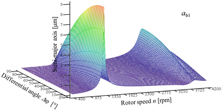
Figure 17. Semi-major axis ab1 of the absolute orbits of the bearing housing point B1.
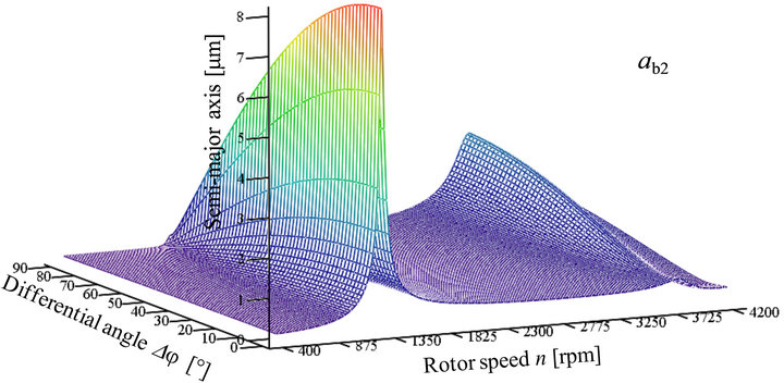
Figure 18. Semi-major axis ab2 of the absolute orbits of the bearing housing point B2.
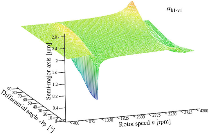
Figure 19. Semi-major axis ab1-v1 of the relative orbits between shaft journal point V1 and bearing housing point B1.
Again two maxima are obvious in each figure. In Figure 19 the maxima occur at a rotor speed of 1255 rpm and at a differential angle of 52˚ with a magnitude of 2.28 μm and at a rotor speed of 3725 rpm and at a differential angle of 90˚ with a magnitude of 2.48 μm. In Figure 20, the maxima occur at a rotor speed of 1312 rpm with a differential angle of 65˚ and a magnitude of 2.21 μm. The second maximum occurs at 3762 rpm with a differential angle of 50˚ and a magnitude of 2.63 μm.
Here the difference between the rotor speeds of the maxima and the critical speeds is a little bit larger. The reason is that a relative movement between two points is analyzed here and not only absolute movements.
Bearing housing vibrations:
The bearing housing vibrations for bearing housing point B1 in horizontal (y-direction) and vertical (z-direction) direction are pictured in Figure 21.
The maxima of the bearing housing vibrations in horizontal direction for bearing housing point B1 (Figure 21(a)) occur at a rotor speed of 1293 rpm and at a differential angle of 0˚ with a magnitude of 0.98 mm/s and at a rotor speed of 3820 rpm and at a differential angle of
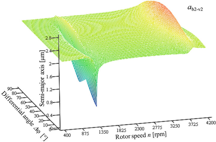
Figure 20. Semi-major axis ab2-v2 of the relative orbits between shaft journal point V2 and bearing housing point B2.
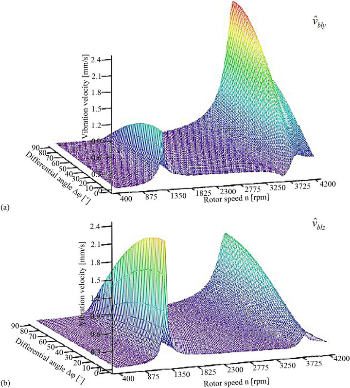
Figure 21. Bearing housing vibrations of bearing housing point B1: (a) Horizontal direction; (b) Vertical direction.
90˚ with magnitude of 2.39 mm/s. The maxima for vertical direction (Figure 21(b)) occur at the same rotor speeds and at the same differential angle, but with different magnitudes. For vertical direction, the maximum occurs now at the low speed (1293 rpm) with a magnitude of 2.04 mm/s. At a rotor speed of 3820 rpm the magnitude is 1.18 mm/s. The bearing housing vibrations for bearing housing point B2 (Figure 22) look similar in comparison to bearing housing vibrations for bearing housing point B1 (Figure 21).
The maxima of the bearing housing vibrations for bearing housing point B2 occur at the same rotor speeds as for bearing housing point B1. For horizontal direction the maxima are 0.93 mm/s at a rotor speed of 1293 rpm and at a differential angle of 0˚, and 1.76 mm/s at a rotor speed of 3820 rpm and at a differential angle of 90˚. For vertical direction the maxima are 1.92 mm/s at a rotor speed of 1293 rpm and at a differential angle of 0˚ and 0.81 mm/s at a rotor speed of 3820 rpm and at a differential angle of 90˚.
For the analysis of the bearing housing vibrations, the rotor speeds of the maxima nearly coincide again with the critical speeds nc2 and nc3 of Figure 12.
4.3. Discussion of the Results
By analyzing the vibration results it can be stated, that without considering the mass moments of inertia of the rotor and therefore without considering the gyroscopic effect only one maximum at low speed would have been found. The maximum at the high speed would not have been found. By considering the mass moments of inertia and the gyroscopic influence, two critical speeds have been found instead of only one critical speed, when neglecting the mass moments of inertia and therefore also the gyroscopic effect. This is exemplarily shown in Figure 23, where the bearing housing vibrations of the bearing housing point B1 is shown, without considering the mass moments of inertias of the rotor (Θp = Θa = 0) and therefore without considering the gyroscopic effect.
When comparing Figure 23 with Figure 21, it can be stated, that the maxima for the first resonance—occurring at the same rotor speed (1293 rpm)—are nearly completely identical. Therefore, the influence of the mass moments of inertia and the gyroscopic effect on the first resonance can be neglected here. However, no second resonance is obvious in Figure 23, because of the ne-

Figure 22. Bearing housing vibrations of bearing housing point B2: (a) Horizontal direction; (b) Vertical direction.
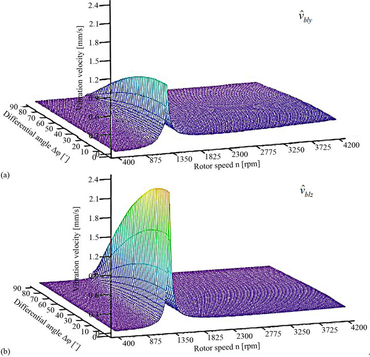
Figure 23. Horizontal (a) and vertical (b) bearing housing vibrations of bearing housing point B1 without considering the mass moments of inertia of the rotor (Qp = Qa = 0).
glected mass moments of inertia. So here the mass moments of inertia and the gyroscopic effect determine the second resonance in Figure 21.
In all diagrams in Section 4.2, it is obvious that, if the orientation of the ellipses of the shaft journals is identical (Dj = 0˚), mode 4 (Figure 13) can be excited easily. However, if the orientation is orthogonal (Dj = 90˚), mode 5 (Figure 13) can be excited more easily.
5. Conclusion
The paper presents a mathematical rotordynamic model regarding excitation due to elliptical shaft journals in sleeve bearings of electrical motors, also considering the gyroscopic effect. It was shown that elliptical shaft journals lead to a forced movement of the shaft journals on the oil film of the sleeve bearings resulting in an excitation of the rotordynamic system. For this kind of excitation a mathematical rotordynamic model was developed considering the influence of the oil film stiffness and damping of the sleeve bearings, the stiffness of the endshields and bearing housings, the stiffness of the rotor, the electromagnetic stiffness in the air gap of the electrical motor—radial and angular electromagnetic stiffness— the mass moment of inertia and the gyroscopic effect of the rotor. The solution of the linear differential equation system leads to the mathematical description of the absolute orbits of the shaft centre, the shaft journals and the bearing housings, and to the relative orbits between the shaft journals and the bearing housings. Additionally, the bearing housing velocities can be computed.
REFERENCES
- M. I. Friswell, J. E. T Penny, S. D. Garvey and A. W. Lees, “Dynamics of Rotating Machines,” Cambridge University Press, Cambridge, 2010.
- J. S. Rao, “Rotor Dynamics,” John Wiley & Sons, New York, 1996.
- R. Gasch, R. Nordmann and H. Pfützner, “Rotordynamik,” Springer-Verlag, Berlin-Heidelberg, 2002.
- A. C. Smith, D. G. Dorrell, “Calculation and Measurement of Unbalanced Magnetic Pull in Cage Induction Motors with Eccentric Rotors, I. Analytical Model,” Proceedings of Electric Power Applications, Vol. 143, No. 3, 1996, pp. 193-201.
- W. Schuisky, “Magnetic Pull in Electrical Machines Due to the Eccentricity of the Rotor,” Electrical Research Association Translation, Vol. 295, 1972, pp. 391-399.
- R. Belmans, A. Vandenput and W. Geysen, “Calculation of the Flux Density and the Unbalanced Pull in Two Pole Induction Machines,” Archiv der Elektrotechnik, Vol. 70, Springer-Verlag, 1987, pp. 151-161.
- R. L. Stoll, “Simple Computational Model for Calculating the Unbalanced Magnetic Pull on a Two-Pole Turbogenerator Rotor Due to Eccentricity,” IEE Proceedings of Electric Power Applications, Vol. 144, No. 4, 1997, pp. 263-270. doi:10.1049/ip-epa:19971143
- T. P. Holopainen, “Electromechanical Interaction in Rotor Dynamics of Cage Induction Motors,” VTT Technical Research Centre of Finland, Ph.D. Thesis, Helsinki University of Technology, Helsinki, 2004.
- H.-O. Seinsch, “Oberfelderscheinungen in Drehfeldmaschinen,” Teubner-Verlag, Stuttgart, 1992.
- U. Werner, “Rotordynamische Analyse von Asynchronmaschinen mit Magnetischen Unsymmetrien,” Dissertation, Technical University of Darmstadt, Darmstadt, 2006.
- U. Werner, “Rotordynamic Model for Electromagnetic Excitation Caused by an Eccentric and Angular Rotor Core in an Induction Motor,” Archive of Applied Mechanics, 2013. doi:10.1007/s00419-013-0743-8
- U. Werner, “Theoretical Vibration Analysis Regarding Excitation Due to Elliptical Shaft Journals in Sleeve Bearings of Electrical Motors,” International Journal of Rotating Machinery, Vol. 2012, 2012, Article ID 860293. doi:10.1155/2012/860293
- O. Reynolds, “On the Theory of Lubrication,” Philosophical Transaction of the Royal Society, Vol. 177, London, 1886.
- J. Lund and K. Thomsen, “A Calculation Method and Data for the Dynamics of Oil Lubricated Journal Bearings in Fluid Film Bearings and Rotor Bearings System Design and Optimization,” ASME, New York, 1978, pp. 1- 28.
- A. Tondl, “Some Problems of Rotor Dynamics,” Chapman & Hall, London, 1965.
- A. A. Gnandoss and M. R. Osborne, “The Numerical Solution of Reynolds’ Equation for a Journal Bearing,” Quarterly Journal of Mechanics and Applied Mathematics, Vol. 17, No. 2, 1964, pp. 241-246. doi:10.1093/qjmam/17.2.241
- J. Glienicke, “Federund Dämpfungskonstanten von Gleitlagern für Turbomaschinen und deren Einfluss auf das Schwingungsverhalten eines Einfachen Rotors,” Dissertation, Technische Hochschule Karlsruhe, Karlsruhe, 1966.
- IEC 60034-14, “Rotating Electrical Machines—Part 14: Mechanical Vibration of Certain Machines with Shaft Heights 56 mm and Higher—Measurement, Evaluation and Limits of Vibration Severity,” International Electrotechnical Commission, 2007.
- ANSI/API 541, “Form-Wound-Squirrel-Cage Induction Motors-500 Horse Power and Larger,” API, 2004.
1. Appendix
1.1. Coefficients of the Mass Matrix M
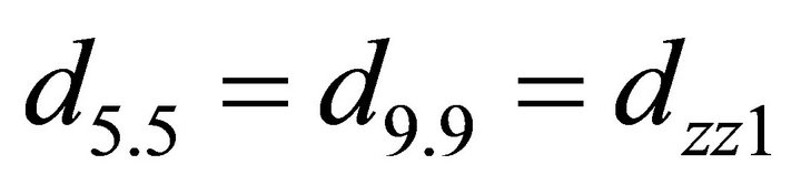
 ;
; 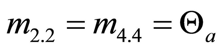
The other coefficients of the matrix are zero.
1.2. Coefficients of the Gyroscopic Matrix G
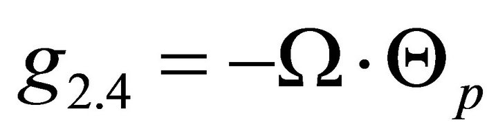 ;
; 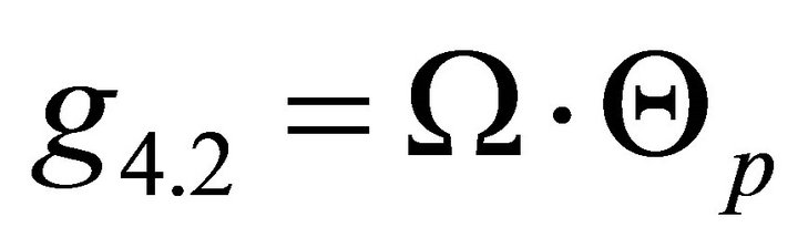
The other coefficients of the matrix are zero.
1.3. Coefficients of the Damping Matrix D
 ;
;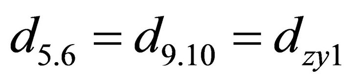 ;
;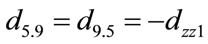 ;
;
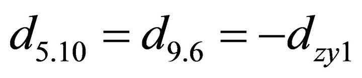 ;
;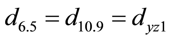 ;
; 
 ;
; ;
;
 ;
; ;
;
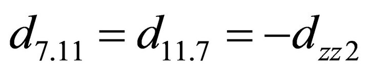 ;
;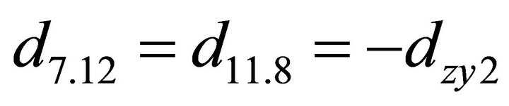 ;
;
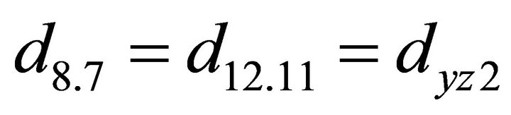 ;
;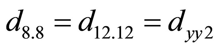 ;
;
 ;
; 
The other coefficients of the matrix are zero.
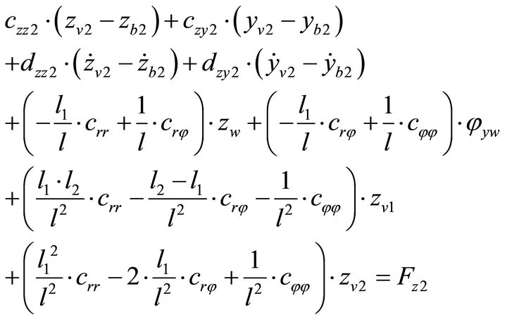
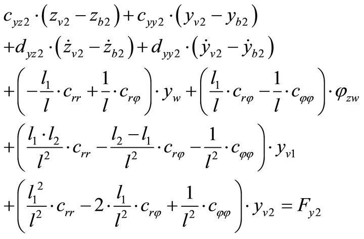
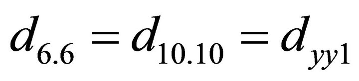
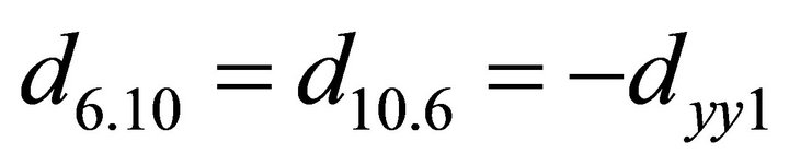
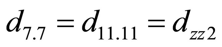
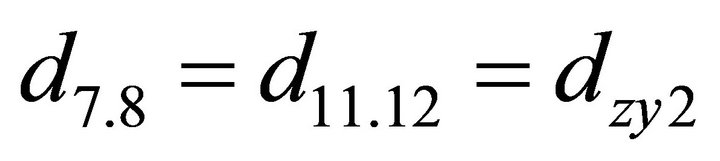
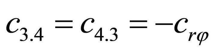
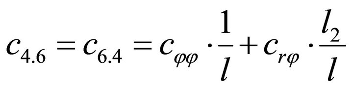
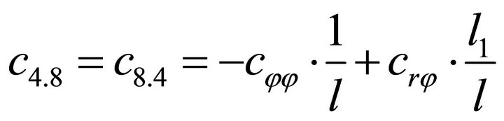
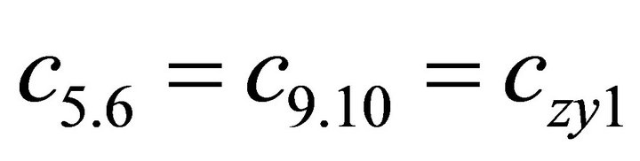
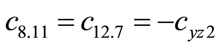
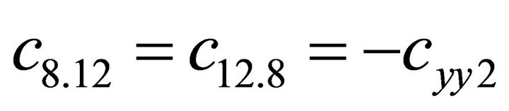
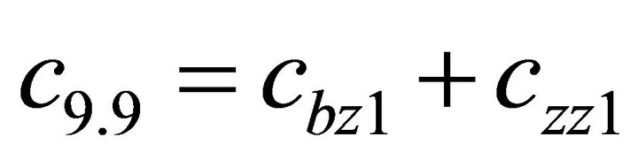
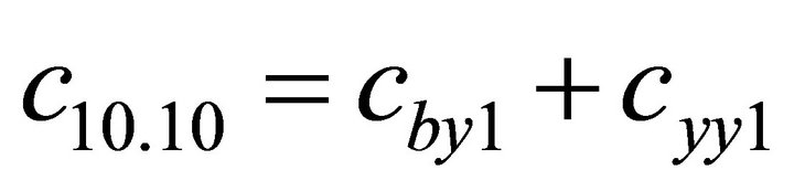
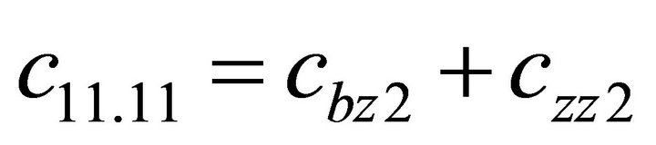
1.4. Coefficients of the Stiffness Matrix C
 ;
; 
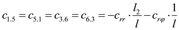
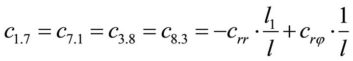
 ;
; 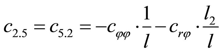
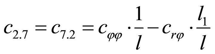 ;
; 
 ;
; 
 ;
; 
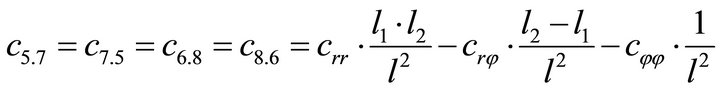
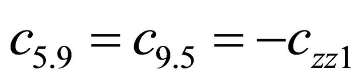 ;
;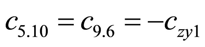 ;
; 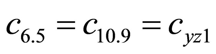
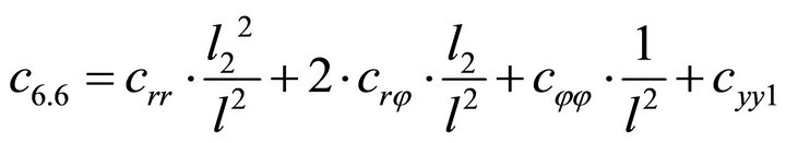 ;
;
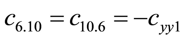
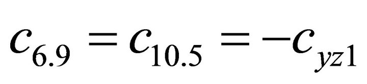 ;
;
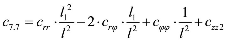
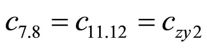 ;
; ;
;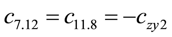
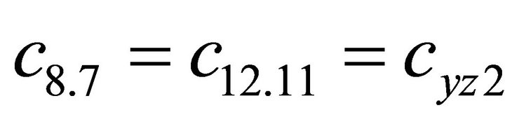 ;
; 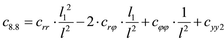
 ;
; ;
;
 ;
; ;
;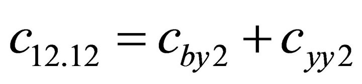
The other coefficients of the matrix are zero.