Applied Mathematics
Vol. 4 No. 8 (2013) , Article ID: 35332 , 5 pages DOI:10.4236/am.2013.48156
Implementing Lagrangean Decomposition Technique to Acquire an Adequate Lower Boundon the Facility Location Problem Solution
Department of Mathematics, College of Basic Education Public Authority for Applied Education and Training, Kuwait City, Kuwait
Email: *rihabfadil@gmail.com
Copyright © 2013 Eiman Jadaan Alenezy, Rehab F. Khalaf. This is an open access article distributed under the Creative Commons Attribution License, which permits unrestricted use, distribution, and reproduction in any medium, provided the original work is properly cited.
Received November 10, 2012; revised January 2, 2013; accepted January 9, 2013
Keywords: Capacitated Facility Location Problem; Lagrangean Relaxation Technique; Volume Algorithm; Randomised Rounding Technique; Unit Cost Technique
ABSTRACT
In this work, the Lagrangean Relaxation method has been discussed to solve different sizes of capacitated facility location problem (CFLP). A good lower bound has been achieved on the solution of the CFLP considered in this paper. This lower bound has been improved by using the Volume algorithm. The methods of setting two important parameters in heuristic have been given. The approaches used to gain the lower bound have been explained. The results of this work have been compared with the known results given by Beasley.
1. Introduction
Due to its wide applications, capacitated facility location problem (CFLP) has been studied by several authors including Holmberg et al. [1], Melkote & Daskin [2], Ahuja et al. [3], Cortinhal & Captivo [4], Contreras & Diaz [5], and Leitner, M., Raidl, G.R. [6]. A much known goal in CFLP research area is to minimize the overall cost associated to a specific way of opening up facilities and serving customers.
The Lagrangean Decomposition technique has been used widely since Held and Karp [7] introduced it. The basic idea of Lagrangean Relaxation or Lagrangean Decomposition is relaxing some constrains in order to eliminate their effect. The motivation for the relaxing of these constrains is that many combinatorial optimization problems consist of an easy problem with some additional complicating constraints. So, relaxing these complicating constrains makes the problem much easier to solve.
This work implements the Lagrangean Decomposition technique to obtain a good lower bound, then the Volume algorithm used to improve this lower bound. Also the Unite Cost Technique is used, then after 50 passes, we switch to use the Randomised Rounding Technique. Moreover, the Randomised Rounding Technique and the Unit Cost Technique have been implemented to solve the facility location problem considered in this paper.
The rest of this paper is organized as the following: the notations, definitions and abbreviation used in this paper are listed in Section 2. In Section 3, the mathematical formulation of location problem is described. A clear explanation of the Lagrangean Relaxation and Lagrangean Decomposition are given in Sections 4 and 5 respectively. The steps of Volume algorithm have been given in Section 6. The approaches of computing the lower bound and the upper bound are given in Section 7. In Section 8, clear descriptions for the Randomised Rounding Technique and the Unit cost technique are given. In Section 9, the tables of the results and comparison are presented. The conclusions are given in Section 10.
2. Notations and Definitions
In the rest of this paper, the following list of notations, definitions and abbreviation is considered:

3. Mathematical Formulation of Location Problem
The formulation of the CFLP as a mixed-integer programing problem called (IP) is given in Equations/Inequalities (1) to (7)
 (1)
(1)
where this is the objective equation
 (2)
(2)
This equation ensure that the demand of each customer is satisfied
 (3)
(3)
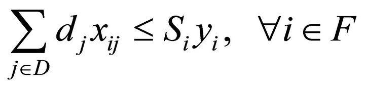
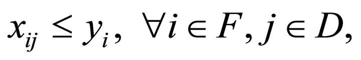
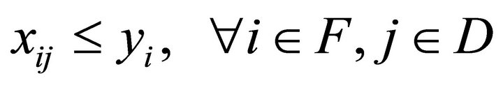 (4)
(4)
These two inequalities ensure that the closed facility does not supply any customer and that the demand supplied from facility does not exceed the capacity of the facility.
 (5)
(5)
This is the integrality constraint.
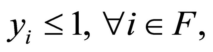
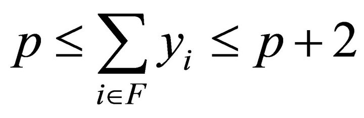 (6)
(6)
This inequality ensure that the number of open facilities lies between p and p + 2, where these constrains were discussed in previous work of the first author, see Alenezy E. [8].
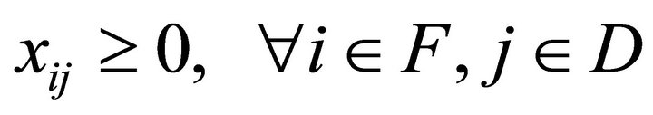 (7)
(7)
The last inequality provide bounds on the allocation variables .
.
4. Lagrangean Relaxsation Technique (LR)
In order to develop a Lagrangean heuristic for the CFLP mentioned in the previous section, a linear programming relaxation for the (IP) problem should be considered, so the same formulation (IP) has to be used except replacing inequality (5) by:
 (8)
(8)
The LP-relaxation will be denoted by (P).
In this section, the Lagrangean relaxation is considered for the problem (P). Then it is described how to use the Volume algorithm, which is an extension to the subgradient Optimisation, Held et al. [9].
Investigating the solution of large sized problems in order to solve the CFLP required decomposing it into m independent problems, which are easier to solve. So we need to relax the most complicated constraint for decomposition, then we relax Equation (2).
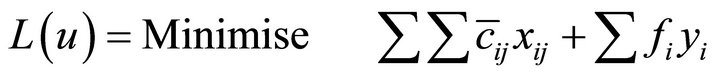
Let uj be the dual multiplier form j Inequation (2), and let . Then a lower bound
  is given by solving the following problem:
 (9)
(9)
 (10)
(10)
 (11)
(11)
 (12)
(12)
 (13)
(13)
 (14)
(14)
5. Lagrangean Decomposition Technique (LD)
From the literature review, it is reported that solving the above , provide an adequate lower bound on the integer optimum solution. This is improved by using the Volume algorithm.
Also from the literature review it is a fact that solving  for large size problems is difficult. To compute a lower bound (LB), we relax constraint (13) and decompose the
  problem into m independent problems for each
 . The generic form of each subproblem is:
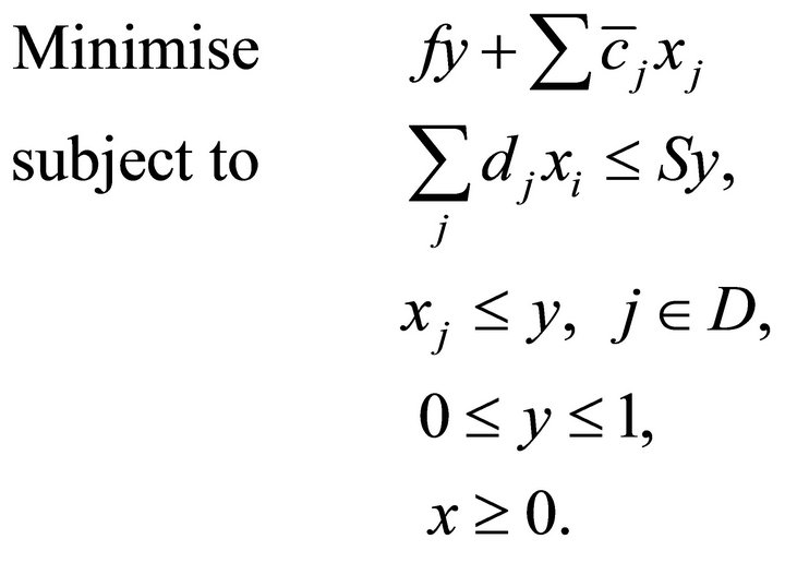 (15)
(15)
Solving this to get a LB is easy. First, set any variable xj with , to 0. Then we assume that the rest of the variables are ordered such that:
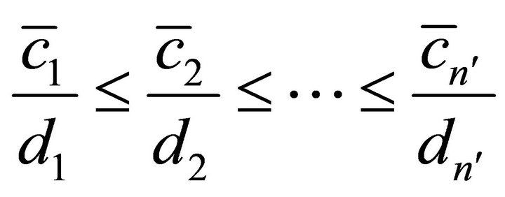 where
where  and
and 
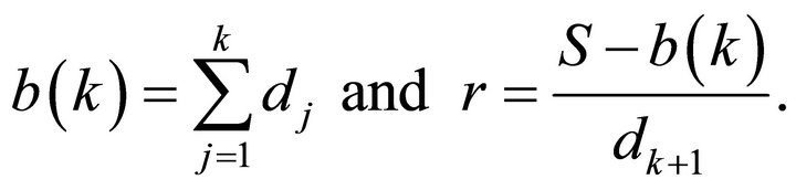
Now, let k be the largest index such that

and let
If 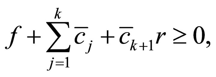 then we set
  and
and  for all j. otherwise, we set

Having solved these m independent subproblems, next, consider the minimum number of facilities that are needed to supply all the demand. In this way the LB enhanced by comparing the number of open facilities denoted by h, after having solved the m subproblems, to the minimum needed p. If , then we sort the unopened facilities by their fixed costs and open the cheapest facilities until we have p opened. The LB is suitably increased to account for theses extra fixed costs.
6. The Volume Algorithm
The Volume algorithm has been used to improve the lower bound obtained from solving the decomposition of the problem in the previous section. The volume algorithm developed by Barhommna and Anbil [10], and it can be described by the following steps:
Step 1: Start with a vector ![]() and solve Equations/ Inequalities (9) to (14) to obtain
and solve Equations/ Inequalities (9) to (14) to obtain  and
and  set
set .
.
Step 2: Compute , where
 , and
, and .
.
The formula of the step size s given by
 (16)
(16)
where this formula is used in the Subgradient method, see (Serra D. [11]).
![]() is a number between 0 and 2. In order to set its value, we will define three types of interations:
is a number between 0 and 2. In order to set its value, we will define three types of interations:
1) Interation E: which is the interation with no improvement on the lower bound. A sequence of E interations requires the need for a smaller step size. Therefore, after a sequence of 20 E interations, we multiply ![]() by 0.66.
by 0.66.
2) Interation Y: if , we compute
 for all j, and
 . If
. If  this means that a larger step size would have a smaller value for
 .
.
3) Interation T: if , this interation suggests the need for a large step size, so we multiply
 ![]() by 1.1.
by 1.1.
Now solve (9) to (14) with . Let
. Let  be the solution obtained. Then
  is updated as

where ![]() is a number between 0 and 1. In order to find the value of
is a number between 0 and 1. In order to find the value of![]() , we solve the following one dimensional problem:
, we solve the following one dimensional problem:
Originally b is set to 0.1, and then every 100 interations we check if  had not increased by at least 1%, in which case we divide b by 2, otherwise we keep it as it is. When b becomes less than 10−5, we keep it constant at this value.
Step 3: Update ![]() as
as  only if
 .
.
Step 4: Stopping criteria 1) .
.
2) .
.
3) The number of passes = 200.
4) If stopping rules are not satisfied, then set  and go to Step 2.
7. Computing the Lower Bound (LB) and the Upper Bound (UB)
7.1. Computing the Lower Bound (LB)
There are two approaches to solve the L(u) formulation of the problem given in Section 4. Following are the summaries of these two approaches:
The First approach summarized by decomposing L(u) in to m independent subproblems. Solve them as explained in Section 5 and update the obtained LB by using the Volume algorithm explained in Section 6, we set the vector ![]() to values that is denoted by “Warm Start Duals”. The Warm Start Duals are the values of the duals of the relaxed constraints (1) and (2) obtained from solving the greedy Weak Representation of the CFLP as LP solution see Alenezy E., et al. [8].
to values that is denoted by “Warm Start Duals”. The Warm Start Duals are the values of the duals of the relaxed constraints (1) and (2) obtained from solving the greedy Weak Representation of the CFLP as LP solution see Alenezy E., et al. [8].
The second approach summarized by removing constrain (11) from the L(u) formulation to reduce the size of the problem to make it possible to solve. Then solve it without the decomposition technique above, to obtain a LB. To improve this LB again, we apply Volume algorithm with the same two ways discussed in the first approach.
7.2. Computing the Upper Bound (UB)
To compute the upper bound, first remove the constraints (4). Solve the (P) formulation for a LP solution. Then use a technique called randomides rounding with new technique called the Unit Cost Technique, these new techniques are explained in Section 8. To treat the fractional solutions of y as a probability distribution, and keep opining them randomly to get enough capacity, we keep updating this UB using the Volume algorithm every 50 passes, until we meet one of the stopping criteria. We choose the passes to be 50, because the UB changes slowly, and from our experiments 50 passes usually shows some improvement in the UB.
8. The Randomised Rounding Technique and the Unit Cost Technique
To describe the Randomised Rounding Technique, let  be the optimal solution to the linear programming relaxation (P) after removing constraints (4). We open facility at location
  with probability
  independently. It is possible that there is not enough total capacity to service all the demand. If this is the case, then we repeat the random experiment and try again. Once we determine which facilities to open, the cheapest of clients can be easily found by solving the resulting transportation problem.
The process of this technique can be summaries as the following:
1) Check if opening all fractional  leads to enough capacity. If not, then open all the
 , and then open the other
  randomly until enough capacity is obtained.
2) If the fractional providing enough capacity, we normalise the fractional
 , so that the sum to 1. Then using this as a probability distribution of the
 . We use the inverse transformation method to select facilities to open until we have enough capacity.
In the Unit Cost Technique, all the  sorted according to their unit cost, which is the value of (fixed cost/capacity) for each unopened facility. We start opening the facility with the cheapest cost until we reach the point where the total capacity exceeds the total demand. In this situation, we sort the remaining facilities in ascending order of the fixed costs and open the first facility in this order list that provides enough capacity to cover the outstanding demand.
9. Problems and Their Tables
The Lagrangean Relaxation implemented in FortRAN, with FortMP as a solver when applicable. The performance of the Lagrangean Relaxation and Volume algorithm have been tested on different problems by using alternative benchmark models.
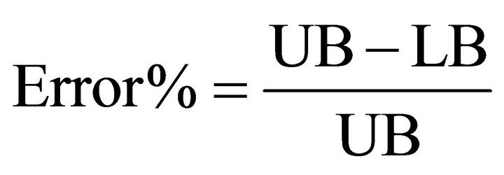
The results of our experiments are given in the following tables. The column “Passes” presented the number of time we go through the algorithm looking for better Lower bound and upper bound. The last row corresponds to the error percentage value which shows the percentage gap between the lower and the upper boundwhere
In Table 1, we use eight instances generated as in the work of Barahona and Anbil [10], and the work of Cornuejols et al. [12].
In Table 2, Beasly’s test problem has been considered and solved using the method of this work. Comparing our solutions with Beasley’s, we notice that we were able to obtain a very close solution of Beasley’s where the reason is using different machines to get the solutions see (Beasley [13]). The gap between our solutions and Beasley’s is less than 1%.
10. Conclusion
A good lower bound has been achieved on the solution of the Capacitated Facility Location Problem considered in
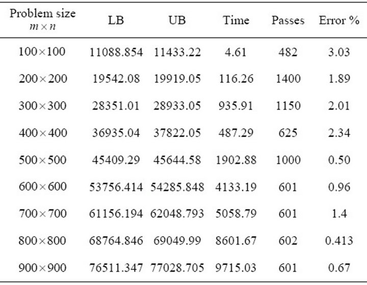
Table 1. The results of solving different size of CFLB problem using Lagrangean Relaxation Technique and Volume algorithm.

Table 2. Comparing the results obtain using Lagrangean Relaxation Technique and Volume algorithm with Beasley results.
this work. The Volume algorithm has been used to improve the lower bound.
REFERENCES
- K. Holmberg, M. Ronnqvist and D. Yuan, “An Exact Algorithm for the Capacitated Facility Location Problems with Single Sourcing,” European Journal of Operational Research, Vol. 113, No. 3, 1999, pp. 544-559. doi:10.1016/S0377-2217(98)00008-3
- S. Melkote and M. S. Daskin, “Capacitated Facility Location-Network Design Problems,” European Journal of Operational Research, Vol. 129, No. 3, 2001, pp. 481- 495. doi:10.1016/S0377-2217(99)00464-6
- R. K. Ahuja, J. B. Orlin, S. Pallottino, M. P. Scaparra and M. G. Scutella, “A Multiexchange Heuristic for the Single-Source Capacitated Facility Location Problem,” Management Science, Vol. 50, No. 6, 2004, pp. 749-760. doi:10.1287/mnsc.1030.0193
- M. J. Cortinhal and M. E. Captivo, “Genetic Algorithms for the Single Source Capacitated Location Problem,” Metaheuristics: Computer Decision-Making, Vol. 86, 2004, pp. 187-216.
- I. A. Contreras and J. A. Diaz, “Scatter Search for the Single Source Capacitated Facility Location Problem,” Annals of Operations Research, Vol. 157, No. 1, 2008, pp. 73-89. doi:10.1007/s10479-007-0193-1
- M. Leitner and G. R. Raidl, “A Lagrangian Decomposition Based Heuristic for Capacitated Connected Facility Location,” In: S. Voß and M. Caserta, Eds., Proceedings of the 8th Metaheuristic International Conference (MIC 2009), Hamburg, 13-16 July 2009.
- M. Held and R. M. Karp, “The Travelling Salesman Problem and Minimum Spanning Trees,” Operations Research, Vol. 18, No. 6, 1970, pp. 1138-1162. doi:10.1287/opre.18.6.1138
- E. J. Alenezy, “Practical Techniques to Solve Capacitated Facility Location Problem,” Far East Journal of Mathematical Sciences (FJMS), Vol. 37, No. 1, 2010, pp. 49-60.
- M. Held, C. Wolf and H. Crowder, “Validation Subgradient Optimisation,” Mathematical Programming, Vol. 6, No. 1, 1974, pp. 62-88. doi:10.1007/BF01580223
- F. Barahona and R. Anbil, “The Volume Algorithm: Producing Primal Solutions Using a Subgradient Method,” Mathematical Programming, Vol. 87, No. 3, 2000, pp. 385-399. doi:10.1007/s101070050002
- D. Serra, S. Ratick and C. Revelle, “The Maximum Capture Problem with Uncertainty,” Environment and Planning, Vol. B23, No. 1, 1996, pp. 49-59.
- G. Cornuejols, R. Sridharn and J. Thizy, “A Comparison of Heuristics and Relaxations for the Capacitated Plant Location Problem,” European Journal and Opertional Research, Vol. 50, No. 3, 1991, pp. 280-297. doi:10.1016/0377-2217(91)90261-S
- J. E. Beasley, (1990), “Distributing Test Problems by Electronic Mail,” Journal of the Operational Research Society, Vol. 41, No. 11, 1990, pp. 1069-1072.
NOTES
*Corresponding author.