Applied Mathematics
Vol.3 No.12(2012), Article ID:25447,6 pages DOI:10.4236/am.2012.312259
Bayesian Markov Regime-Switching Models for Cointegration
1Department of Statistical Science, Duke University, Durham, USA
2School of Science and Information, Qingdao Agricultural University, Qingdao, China
Email: kc52@stat.duke.edu, wshcui@qau.edu.cn
Received October 10, 2012; revised November 11, 2012; accepted November 18, 2012
Keywords: Cointegration; Regime-Switching; Bayesian; MCMC
ABSTRACT
This paper introduces a Bayesian Markov regime-switching model that allows the cointegration relationship between two time series to be switched on and off over time. Unlike classical approaches for testing and modeling cointegration, the Bayesian Markov switching method allows for estimation of the regime-specific model parameters via Markov Chain Monte Carlo and generates more reliable estimation. Inference of regime switching also provides important information for further analysis and decision making.
1. Introduction
Since the development of the concept of cointegration [1], there has been a rich literature on testing cointegration and applying cointegration approaches to real data analysis. One of the most illustrative examples in practice is the pair trading strategy [2]. The basic idea is that: find two securities whose prices have been historically moving together. So when the spread between them widens, we short the winner and buy the loser. And if we believe that the history would repeat itself, prices will converge again and the arbitrager will profit. This moving-together relationship between two nonstationary time series is called cointegration. Mathematically, if two nonstationary time series  and
and  are cointegrated, then there exists a number
 ![]() called the cointegration ratio, such that
called the cointegration ratio, such that  is stationary.
Although there have been many statistical studies to find cointegrated time series, there are still many unsolved problems. First of all, it is often hard simply to find cointegration given a specific period of time. There are several statistical explanations for failing to reject the null of no cointegration including the span of the data set, structural breaks [3] and the choice of test model [4]. Secondly, there are few statistical decision-making rules after identifying candidate pairs. Taking pair trading as an exmple, typically, people simply use the decision rule that they open a long-short position when the pair prices have diverged by a certain amount (e.g. two standard deviations from the historical mean) and close the position when the prices have reverted [5].
This paper proposes the Bayesian Markov regimeswitching model that allows the cointegration relationship between two time series to be switched on or off over time via a discrete-time Markov process. This is an improvement to the traditional cointegration tests considering that the model flexibly allows local non-cointegration rather than assuming global cointegration over the whole period of time. By using a fully Bayesian models, uncertainty about cointegration ratio is also incorporated into the model and inferred simultaneously with all other unknown quantities. Furthermore, inference of the hidden regime-switching is also critical to decision making and further generic analysis.
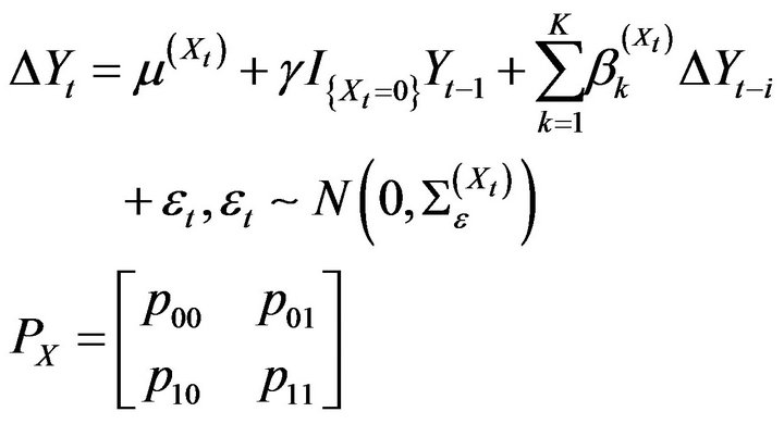
2. Markov Regime-Switching Models for Cointegration
Suppose we have two nonstationary time series  and
and  with integration order 1, and
  (
(![]() is known, typically people propose a
is known, typically people propose a ![]() and then test the stationary property of
and then test the stationary property of![]() ). If
). If ![]() is stationary, then we say time series
is stationary, then we say time series  and
and  are cointegrated. To test for stationarity, the Engle-Grange method [6] tests the
  null hypothesis using the ADF unit root test [5] based on the Error Correction Model (EVM) with lag order K (as compared to
  in which case it is stationary):
 (1)
(1)
where  is a constant,
  s are autoregression coefficients and
 .
.
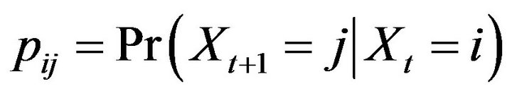
In comparison, the Markov regime-switching model we proposed allows ![]() to switch between cointegrated or non-cointegrated regimes in a Markovian manner, by introducing the regime indicator variable
to switch between cointegrated or non-cointegrated regimes in a Markovian manner, by introducing the regime indicator variable , regime specific parameters and the Markov transition matrix
 . For the simplicity of exposition, we assume that
 , with
  denoting that that
 ![]() is stationary (i.e.
is stationary (i.e.  and
and  are cointegrated) at time t and
  meaning non-cointegration. Then the model can be written as:
 (2)
(2)
where  and thus
 .
.  is the Markov transition matrix of
 , with
and initial value .
.
Clearly, when  the model reduces to model (1) with negative
![]() , while
, while  specifies unit root process for
 ![]() and thus no cointegration exists for time series
and thus no cointegration exists for time series  and
and . By obtaining inference of the underlining regimes
 , regime-specific parameters and segmentation of regime-specific data, the model provides much information for further generic analysis and decision making.
3. Bayesian Computation
We propose to use Bayesian analysis for the inference of parameters and latent regimes , where posterior samples of all unknown quantities are drawn using Markov Chain Monte Carlo (MCMC).
Under this model (2), the likelihood function is:

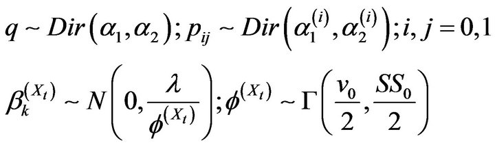
Conjugate prior distributions are placed on model parameters [7]. Specifically, conjugate Dirichlet priors are assigned to each row of the transition matrix  and
and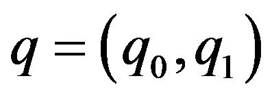 , where
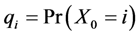 . Conjugate Normal-Gamma priors are assigned for all the regression coefficients
  and the corresponding precisions
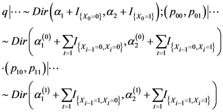
To obtained the posterior marginal distributions of the unknown parameters and the hidden regimes , Gibbs sampler is constructed to iterate the following steps:
1) Sample  and
and  from full conditional distributions:
2) Sample the regression coefficients  and variance from Normal-Inverse Gamma full conditional distributions given the conjugacy of the priors.
3) Sample the whole path of .
.
Since  s are highly correlated, Gibbs sampler constructed via regular full conditional distribution would be extremely inefficient [7]. To overcome this, Forward Filtering and Backward Sampling algorithm is applied to draw block samples of
 . To achieve this, define
 , then by recursion:
and

With this, the results follow that:
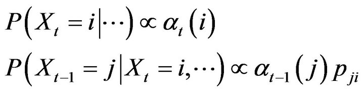
By using this algorithm, a sample of  is first drawn from a bernoulli (multinomial if
  takes more than two values) distribution, and
 , samples of
  are drawn sequentially and backward from the conditional bernoulli distribution, with
 until the whole
 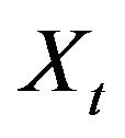 time series are sampled.
4. Simulated Time Series Analysis
4.1. Model Assessment
To testify the performance of the proposed framework, we simulated a Markov regime-switching times series of length , which switches between one stationary AR(2) process (State 0) and one non-stationary AR(2) process (State 1). The two AR(2) models and the corresponding Error Correction Models (ECM) are shown as follows: (the (non-)stationary property can be easily tested by the Unit Root Test)
 (3)
(3)
where . The transition matrix is specified as
 .
.
A simulated data was shown in Figure 1.
The proposed model was applied to the time series to find regime switching, with the priors specified as follows:
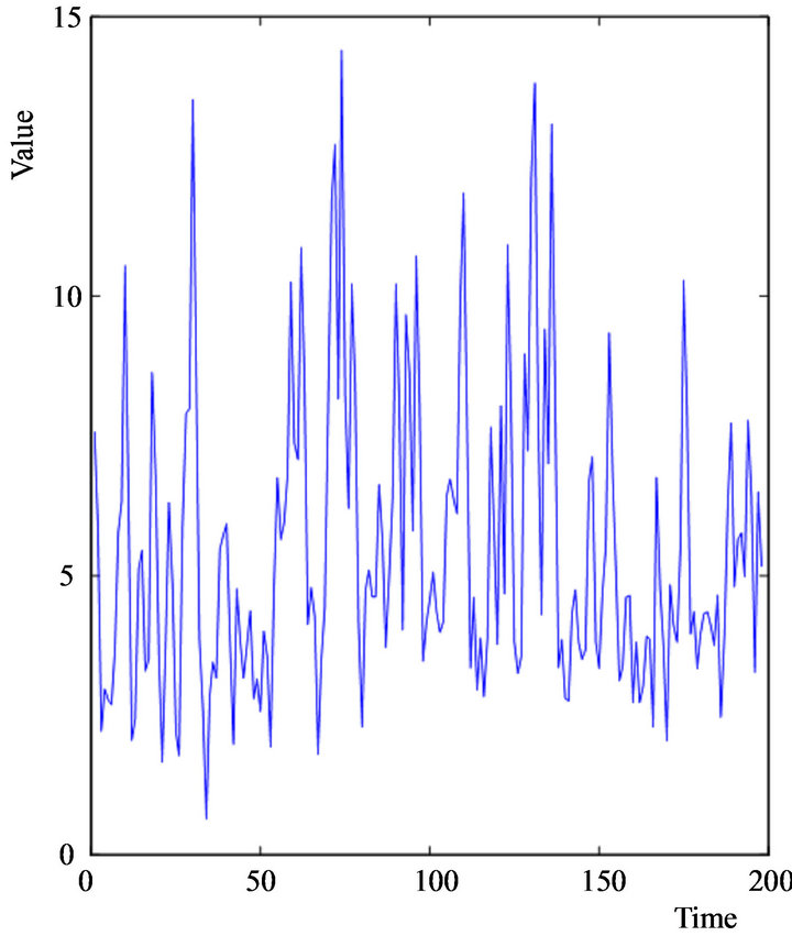
Figure 1. Illutration of a time series stimulated by the markov switching model.
To infer the value of  based on posterior samples, we use posterior probability
  as the cut-off point. Shown in Figure 2, the inferred regimes are compared with the true values, which shows that our model gives good recovery of the latent regimes (with the first 200 time points shown). Other model parameters are also correctly inferred as shown in Table 1, where posterior distributions cover the true values well.
4.2. Posterior Decision Making
The importance of inference of regimes when analyzing (non)stationary time series lies in the fact that commonly-used stationarity and cointegration tests (e.g. ADF unit root test and Engle-Granger cointegration tes [1]) may well give misleading results when regime switching
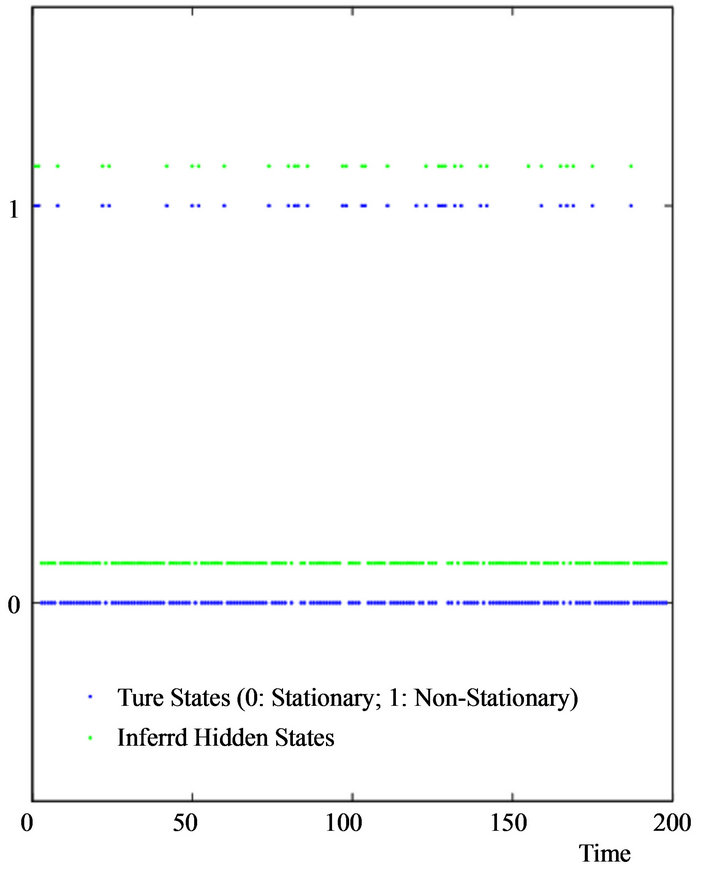
Figure 2. Inferred regimes Xt (in green) compared to the true values (in blue) show good inference.
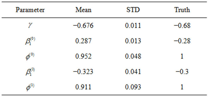
Table 1. Posterior estimates of model parameters compared to the true values. The parameters are defined as in model 2 and specified in (3).
exists in the process. For illustration, a quick ADF test of the previously simulated data concludes that the null hypothesis with unit root is rejected at 99.9% confidence level, indicating the times series is stationary. If this time series were generated by the linear combination of two nonstationary time series, then the ADF test tells that these two are co-integrated, which is clearly wrong.
In the following part, we will use the context of pair trading to illustrate how the Markov regime-switching model can potentially help improve decision making in practice. Basically people do pair trading based on the traditional rule that you open a long-short position when the pair prices have diverged by more than two historical standard deviations. And you unwind the position when it returns to historical mean.
First of all, the model clearly allows more reasonable estimation of the historical mean and standard deviation, based soly on data in the stationary (cointegrated) regimes, rather than including data in the nonstationary (non-cointegrated) regimes. This difference can be observed in Figure 3, where the historical mean using data in the stationary regime is different from that using all data, and the standard deviation is also smaller.
Secondly, the identification of stationary (cointegrated) and nonstationary (non-cointegrated) regimes also help establish more rational decision making rules, which should be: we open a position when it is both in the stationary state and has diverged from the historical stationary mean. It is apparently risky either to open a position when currently we are in a non-stationary state or the historical mean calculation involves non-stationary data.
Since people care much about the time points where values are at least 2 standard deviations away from the historical mean, the figure shows that the we pick different time points using our model and decision making rules from those obtained using all historical data and traditional rules, which we believe are more reasonable choices. For example, many spikes in Figure 3 are actually not good time points to open the position based on our Markov regime-switching model simply because those spikes are in the non-stationary (non-cointegrated) regime. However in comparison, the traditional approach considers them open positions whenever the values are 2 standard deviations away from the mean, which is a very risky decision not considering the regimes.
5. Cointegrated Price Series Analysis
An possible example of a pair of cointegrated time series is the gold ETF, GLD versus the gold miners ETF, GDX. GLD reflects the spot price of gold, and GDX is a basket of gold-mining stocks. It makes intuitive sense that their

Figure 3. Results comparison between our Bayesian Markov regime-switching model and traditional cointegration test and analysis using all historical data. Red lines indicate the mean and mean ±2SD using all historical data, which is a traditional way after you have done the ADF test to show the stationary property; Green lines indicate those using only historical data in stationary regimes. Red and green dots mark the time points where values at those points are at least 2SD away from the historical mean based on traditional and our Markov regime switching model respectively.

Figure 4. Distribution of the probability that Xt is in the cointegration regime (t = 1,···,T).
prices may move in tandem. Previous study via the twostep Engle-Granger method [1] identified that a portfolio with long 1 share of GLD and short 1.6766 share of GDX is likely a stationary time series, with lag 1 but the conclusion is later questioned by other studies [8]. To test the possible co-integration, the two-state Markov regime switching model is applied to the 05/23/06-11/30/07 GLD and GDX time series. A histogram shown the distribution of the probability of the time points being in the cointegration state is shown in Figure 4. According to the previous 0.5 cut-off point, the Markov regime switching model indicates that at most of the time, the two time series are not cointegrated with the 1.6766 cointegration ratio. This may serve as another counterexample (together with the simulation result) that the widely-used ADF test might provide misleading results when used to test co-integration regardless of possible regime switching.
6. Conclusions and Future Work
In this study, we proposed to use the Bayesian Markov regime-switching model as a flexible model for cointegration and stationarity analysis, where the latent regimeswitching process is modeled via a Markov process. A strong message of this study is that, while identifying cointegration (or stationarity) is often hard globally, allowing local non-cointegration (or non-stationarity) and inferring the regime switching can provide much information for further analysis and decision making.
Several extensions of the study are still worth exploring, including relaxing the hidden Markov transition models and incorporating uncertainty about number of regimes in the model. Hidden semi-Markov models are natural extensions of hidden Markov models. While the runlength distribution of the hidden Markov models implicity follows a geometric distribution, hidden semi-Markov models allow for more general runlength distributions, and thus are more flexible to describe the time spend in a given regime. As for the cases with the number of regimes unknown, Bayesian inference through reversible jump MCMC methods [9] could be a viable alternative that both explores models with different number of regimes and estimation of regime-specific parameters.
REFERENCES
- R. F. Engle and C. W. J. Granger, “Co-integration and Error Correction: Representation, Estimation, and Testing,” Econometrica, Vol. 55, No. 2, 1987, pp. 251-276. doi:10.2307/1913236
- H. Puspaningrum, “Pairs Trading Using Cointegration Approach,” Ph.D. Thesis, University of Wollongong, Wollongong, 2012.
- J. Campos and N. R. Ericsson and D. F. Hendry, “Cointegration Tests in the Presence of Structural Breaks,” International Finance Discussion Papers 440, Board of Governors of the Federal Reserve System (US), 1996.
- E. G. Gatev and W. Goetzmann and K. G. Rouwenhorst, “Pairs Trading: Performance of a Relative Value Arbitrage Rule,” Boston College, Boston, 2006.
- A. W. Gregory and B. E. Hansen, “Residual-Based Tests for Cointegration in Models with Regime Shifts,” Journal of Econometrics, Vol. 70, No. 1, 1996, pp. 99-126. doi:10.1016/0304-4076(69)41685-7
- D. A. Dickey and W. A. Fuller, “Distribution of the Estimators for Autoregressive Time Series With a Unit Root,” Journal of the American Statistical Association, Vol. 74, No. 366, 1979, pp. 427-431. doi:10.2307/2286348
- G. E. B. Archer and D. M. Titterington, “Parameter Estimation for Hidden Markov Chains,” Journal of Statistical Planning and Inference, Vol. 108, No. 1, 2002, pp. 365- 390. doi:10.1016/S0378-3758(02)00318-X
- E. P. Chan, “Quantitative Trading,” John Wiley and Sons, Hoboken, 2008.
- C. P. Robert, T. Ryden and D. M. Titterington, “Bayesian Inference in Hidden Markov Models through the Reversible Jump Markov Chain Monte Carlo Method,” Journal of The Royal Statistical Society Series B, Vol. 62, No. 1, 2000, pp. 57-75. doi:10.1111/1467-9868.00219