Applied Mathematics
Vol.3 No.10A(2012), Article ID:24096,13 pages DOI:10.4236/am.2012.330185
Water Supply and Demand Sensitivities of Linear Programming Solutions to a Water Allocation Problem
1Hydrologic Research Center, San Diego, USA
2Scripps Institution of Oceanography, UCSD, La Jolla, USA
Email: KGeorgakakos@hrc-lab.org
Received June 17, 2012; revised July 17, 2012; accepted July 25, 2012
Keywords: Water Allocation; Water Banking; Linear Programming
ABSTRACT
This work formulates and implements a mathematical optimization program to assist water managers with water allocation and banking decisions to meet demands. Linear programming is used to formulate the constraints and objective function of the problem and tests of the developed program are performed with data from the Castaic Lake Water Agency (CLWA) in Southern California. The problem is formulated as a deterministic programming problem over a five year planning horizon with annual resolution. The program accepts annual water allocations from the State Water Project (SWP) in California. It then determines the least-cost feasible allocation of this water toward meeting annual demands in the five-year planning horizon. Local water sources, including water recycling, and water banking programs with their constraints and costs are considered to determine the optimal water allocation policy within the planning horizon. Although there is not enough information to fully account for the uncertainty in future allocations and demands as part of the decision problem solution for CLWA, uncertainty in the SWP allocation is considered in the tests, and sensitivity analyses is performed with respect to demand increases to derive inferences regarding the behavior of the median minimum-cost solutions and of the risk of failure to meet demand.
1. Introduction
The goal of the work is to formulate and test the feasibility of solutions of a mathematical programming problem that will be suitable for annual operation and which will assist Castaic Lake Water Agency (CLWA) with decisions pertaining to meeting demand over a multi-year decision horizon. CLWA was formed in 1962 for the purpose of contracting with the California Department of Water Resources (DWR) to provide a supplemental supply of imported water to four retail water purveyors in the Santa Clarita Valley. CLWA serves an area of 195 square miles in the Los Angeles and Ventura Counties. CLWA and its retail purveyors meet demand through local groundwater pumping, State Water Project water imports, water stored in water banks, and recycled water. The imported water component of the water supply is based on reliability studies conducted and published by the DWR.
There is uncertainty that enters the development of policy over the planning horizon of say N years for CLWA. This uncertainty arises due to future State Water Project (SWP) allocations and due to future demands in the CLWA region. Allocations and demands are influenced by the weather and climate in Northern California and the regional and local weather and climate in the CLWA region and the pattern of regional development. The statistical parameters of this uncertainty are largely unknown at this time to allow a reliable formulation of a stochastic programming problem. Therefore, a deterministic mathematical programming problem formulation is implemented at this time, that is flexible enough to allow for each year the examination of several possible scenarios of SWP allocation and demand (e.g. examination of solutions for a sequence of expected normal years, examination of solutions for possible sequences of dry years, and examination of solution for expected sequences of possible future development). Although the solutions for water to be placed in storage and for water transfers among various storages will be provided for the entire planning horizon, only the present year solution will be implemented as it contains the lowest level of uncertainty. Even this low uncertainty may be considered in the decision process, as CLWA decision makers can examine the spectrum of possible solutions obtained with particular emphasis in any differences for the current year prior to arriving at a decision. An annual time step is used in the formulation.
The next section presents the sources of water supply for the CLWA. Section 3 formulates a linear programming program that includes the constraints pertaining to water supply sources for CLWA and minimizes total cost while meeting demand, Section 4 places the present formulation within the context of the pertinent literature of mathematical programming and application to water resources problems, while Section 5 presents results of application and of sensitivity analysis. Concluding remarks are in Section 6.
2. Sources of Water Supply for CLWA
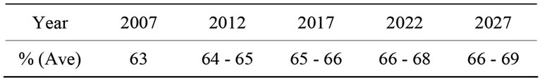
1). Wholesale water imported from SWP: Maximum allocation 95,200 af in any one year. Actual delivery varies in a particular year based on hydrology, amount in SWP storage at the beginning of water year, restrictions in delivery (technological and legal), and total demand requested by SWP contractors. The State Water Project Delivery Reliability Report issued in 2007 (referred to as DWR07 hereafter) shows an average delivery of 66% - 69% of maximum allocation amount under future conditions (set for year 2027). The same report shows an average delivery of 63% of maximum allocation amount under year 2007 conditions (two scenarios of regulatory restrictions in delivery). It also shows average and dry period deliveries under 2007 conditions and future conditions (for year 2027), and the distribution of the percent deliveries discussed above by future years. For instance and for five year intervals, average percent deliveries (maximum allocation amount) are:
With respect to the cost for wholesale SWP water, SWP income from all contractors in 2002 was approximately $600 million for approximately 4.13 million acrefeet (af) of allocated water. CLWA estimated current costs are approximately $110/af per year. In this and subsequent monetary figures we use 2007 US dollars.
2). Flexible storage account in Castaic Lake (Water Supply Contract DWR): CLWA has access to up to 4684 af of the storage in Castaic Lake. This amount must be replaced within 5 years of its withdrawal. CLWA policy is to keep the account full in normal and wet years and then deliver the stored amount or portion during dry years. The account is refilled during the next year that adequate SWP supplies exist to do so. Cost of borrowing consists of the power cost to deliver out of Castaic Lake, while the cost to replace the borrowed amount of water is CLWA’s per af cost plus variable power costs. For this work we assume an annual cost of $120/af per year for deposit and no cost for withdrawal and for storage.
3). Flexible storage account (Ventura County agencies): Access to another 1376 af of storage in Castaic Lake for 10 years beginning in 2006. This amount too must be replaced within 5 years of its withdrawal. Costs for deposit and withdrawal are as in item 2 above plus $15/af per year for storage.
4). Article-21 water: Water available on an unscheduled and interruptible basis for average to wet years, generally only for a limited time. The DWR07 indicates average delivery under 2007 conditions of 90 af and under future conditions (2027) of 30 af. Maximum amounts for 2007 conditions are 590 af and for future conditions are 410 - 420 af. Minimum amounts are 0. It is unlikely that CLWA will utilize this water type in the future.
5). The Turnback Pool: Makes a small amount of water available in all types of hydrologic years (less water in dry years). It depends on urban contractor demand. It is unlikely that CLWA will utilize this water type in the future.
6). DWR Dry Year Water Purchase Programs: DWR purchases from willing sellers in areas of adequate supply and the DWR sells back to those willing to purchase it. This program is not operated in all years and is somewhat uncertain. It is unlikely that CLWA will utilize this water type in the future.
7). Groundwater Alluvium: Governed by hydrologic conditions in eastern Santa Clara River watershed. Pumping ranges 30,000 - 40,000 afy during normal and abovenormal rainfall years. For locally dry years pumping is reduced 30,000 - 35,000 afy (1, 2 or 3 dry year sequences). Annual withdrawal costs are estimated to be $50/af.
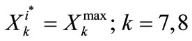
8). Groundwater Saugus Formation: This is linked to the availability of other water supplies in a given year, particularly from the SWP. During average-year conditions within the SWP system, Saugus pumping ranges 7500 - 15,000 afy. Dry year pumping ranges between 15,000 - 25,000 afy during a SWP drought year (reduced SWP deliveries). If SWP deliveries are reduced for 2 consecutive years, pumping can increase to 21,000 - 25,000 afy. If SWP deliveries are reduced for 3 consecutive years, pumping can increase to 21,000 - 35,000 afy. Such high pumping is to be followed by periods of reduced (average-year) pumping rates to recover water levels and groundwater storage. Annual withdrawal costs are estimated to be $150/af.
9). Core transfer (Buena Vista Water Storage District and Rosedale-Rio Bravo Water Storage District): This is a transfer to purchase a defined quantity of water every year, 11,000 afy. Cost is estimated (2005 Urban Water Management Plan—UWMP) to be $60 - $110/afy. In this work, this source of water is used to reduce the demand in all years and it is not part of the optimization problem.
10). Southern water banking programs: Water banking and exchange programs that will provide additional 14,000 af of storage capacity and 6900 af per year of pumpback capacity during a six-month emergency outage. Annual costs are assumed to be $100/af for deposit and $100/af for withdrawal. The storage cost is assumed to be $50/af.
11). Semitropic Water Banking: There is currently a total of 50,870 af stored water, recoverable through 2013 to meet CLWA demands as needed. Current operational planning includes use of the water stored in Semitropic for dry-year supply. Withdrawal costs are $25/af.
12). Rosedale—Rio Bravo Water Storage District Water Banking: A water banking and exchange program with up to 100,000 af storage capacity and pumpback capacity of 20,000 afy. This is to support dry-year supply (not planned growth). Annual storage, deposit and withdrawal costs are $30/af.
13). Recycled water: Table 3-1 of the 2005 UWMP shows 1700 afy. In this work, this source of water is used to reduce the demand in all years and it is not part of the optimization problem.
3. Mathematical Program Formulation
The purpose of the mathematical program formulated in this section is to provide feasible solutions to the water allocation problem for CLWA that are optimal under the set of parameter values used. The mathematical program consists of a set of constraints that define the feasible solutions, and an objective function that facilitates the selection of the “best” feasible solution. For this programming problem, the objective function is an expression of annual costs associated with a certain allocation policy and therefore, in this context the “best” or optimal solution is one that minimizes the objective function. We formulate and interpret the set of constraints and the objective function in the following. It is noted that, for the purposes of this formulation, we adopt an annual time step and a planning horizon of N years. Even though solutions are obtained for all the years in the planning horizon, only the first year solution for the allocation policy is implemented.
3.1. Constraints that Define Feasible Solutions
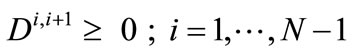
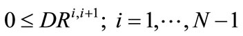
The first set of constraints concerns the State Water Project (SWP) annual allocation to CLWA based on the existing contract between SWP and CLWA. For each year within the planning horizon the constraints assure water volume conservation in the process of delivery, carryover storage and CLWA allocations. The set of constraints is expressed as:
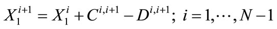 (1)
(1)
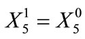
where  represents the SWP carryover storage at the end of time step i (one year in this case),
  is the SWP annual water allocation to CLWA for time step i + 1 (taken as the period from the end of time step i to the end of time step i + 1), and
  is the water used by CLWA during step i + 1 (defined previously) to meet demand at that or future time steps. Due to the fact that carryover storage of a certain year must be used in the next year, the following constraint is used:
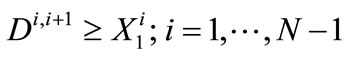 (2)
(2)
The quantity  is program input from actual and/or forecasted SWP allocation (a fraction of the maximum allocation for CLWA, while carryover storage
  and water use by CLWA
  are program solution output. As such, nonnegativity constraints are imposed on the latter two quantities:
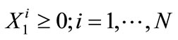 (3)
(3)
 (4)
(4)
while the initial condition on carryover storage  is specified from:
 (5)
(5)
with  known at the beginning of the planning horizon. In addition to the nonnegativity constraints it is also possible to include upper bound constraints for carryover storage
  for all I, but at this time no such constraints are imposed by the CLWA operational policy.
A second set of constraints concerns withdrawals from local groundwater resources (Alluvium and Saugus formation). These constraints are in the form of upper and lower bounds on withdrawals, with the bounds depending on the occurrence of a dry or a medium/wet year. This set of constraints is represented by:
 (6)
(6)
 (7)
(7)
where  is the annual withdrawal from the Alluvium aquifer for period i + 1 (indicated as the period from the end of period i to the end of period i + 1),
  is the analogous annual withdrawal from the Saugus formation,
  signifies the lower bound on the Alluvium aquifer withdrawal for a wet or a dry year in the planning horizon,
  signifies the upper bound on the Alluvium aquifer withdrawal for a wet or a dry year in the planning horizon, and with analogous definitions for the Saugus formation bounds. The values of the bounds are nonnegative and considered known once a certain year in the planning horizon is characterized as wet or dry. This eliminates the need for nonnegativity constraints for the local groundwater withdrawals. The withdrawal amounts
  and
and  for all i are obtained from the solution of the programming program being formulated.
There are three sets of constraints associated with water banking programs that CLWA is currently involved in. The first pertains to the Semitropic bank where CLWA has transferred a significant amount of water already, the second is associated with a groundwater banking program with given constraints of maximum amount stored and maximum annual withdrawal, and the third is associated with the Rosedale— Rio Bravo banking program that has its own constraints pertaining to maximum stored amount and maximum annual withdrawal. These constraints are discussed next for each banking program.
The Semitropic water volume conservation on a year to year basis may be written as:
 (8)
(8)
where  signifies the water mount in Semitropic storage at the end of year i, and
  signifies the annual withdrawal from Semitropic storage for year i + 1 (same notational convention as previously defined for transfer amounts). It is noted that Equation (8) does not include a supply term for Semitropic as it is assumed that CLWA does not intend to increase the water stored in Semitropic. Should this policy change, an additional positive term will be added to the right hand side of Equation (8) to signify annual water amount added to Semitropic storage. Nonnegativity constraints are associated with the Semitropic bank transfers:
 (9)
(9)
 (10)
(10)
and an initial condition is specified for the amount in Semitropic storage at the beginning of the planning horizon:
 (11)
(11)
with  being a known quantity. Lastly, there is a requirement that the amount in storage in Semitropic must be withdrawn by the end of a known year in the future (call it n), and this is enforced by:
 (12)
(12)
The southern water banking programs may be represented by the following constraints (water amount conservation, and bounds on amount stored and on annual amount withdrawn from this bank):
 (13)
(13)
 (14)
(14)
 (15)
(15)
 (16)
(16)
where  signifies the water amount in bank storage at the end of year i,
  signifies the annual withdrawal from bank storage for year i + 1, and
  signifies the annual transfer amount to bank storage by CLWA for year i + 1. The upper bounds for bank storage,
  , and annual withdrawal amount, Bmax, are known quantities, and the unknown quantities whose values result from the solution of the programming problem are the storage amounts (
 ; i = 2, ···, N), and the annual transfer amounts in and out of the southern water bank (
 ,
, ; i = 1, ···, N – 1). The initial storage in the bank at the beginning of the planning horizon is considered known and equal to
 :
:
 (17)
(17)
The analogous constraints for the Rosedale-Rio Bravo banking program are shown below:
 (18)
(18)
 (19)
(19)
 (20)
(20)
 (21)
(21)
 (22)
(22)
where  signifies the water amount in Rosedale-Rio Bravo (RRB) bank storage at the end of year i,
  signifies the annual withdrawal from RRB-bank storage for year i + 1, and
  signifies the annual transfer amount to RRB-bank storage by CLWA for year i + 1. The upper bounds for bank storage,
  , and annual withdrawal amount, Rmax, are known quantities, and the unknown quantities whose values result from the solution of the programming problem are the storage amounts (
 ; i = 2, ···, N), and the annual transfer amounts in and out of the RRB bank (
 ,
, ; i = 1, ···, N − 1). In this case, too, the initial storage in the RRB bank at the beginning of the planning horizon is considered known and equal to
 .
.
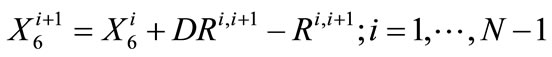
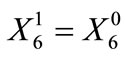
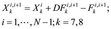
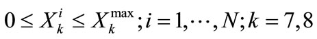
The two Castaic Lake flexible storage accounts mentioned in the water sources section can also be treated as water banks for the purpose of this mathematical formulation. Their separate consideration is necessary because one of the accounts has a 10-year active period while the other does not carry a termination date. The feasibility constraints for the two accounts may be written as:
 (23)
(23)
 (24)
(24)
 (25)
(25)
 (26)
(26)
 (27)
(27)
where k identifies the Castaic Lake flexible storage accounts ( and
and  at the end of year i),
  is the deposit to the kth flexible account for year i + 1,
  is the withdrawal from the kth flexible account for year i + 1, and
  signifies the initial storage in the kth flexible account. Because of the 5-year term refilling conditions prescribed for the flexible accounts additional constraints pertaining to the repayment are imposed:
 (28)
(28)
where i* signifies the end of the year during which refilling of the accounts must be made.
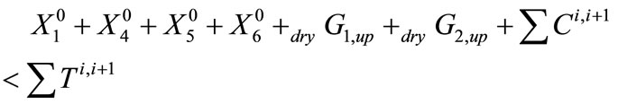
A final set of constraints pertains to meeting demand for each year of the planning horizon:
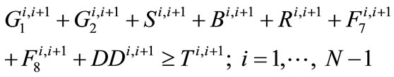 (29)
(29)
where  is the annual demand, considered known.
  is the residual resulting from subtracting the fixed core transfers from Buena Vista Water Storage District (11,000 af) and recycled water (1700 af) from the known regional demand for CLWA. The amount
  is the amount of the SWP allocation to CLWA used directly to satisfy demand, and is constrained by:
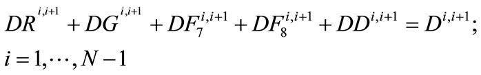 (30)
(30)
and the nonnegativity constraint:
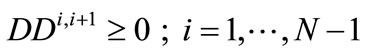 (31)
(31)
This amount ( ) is obtained from the solution of the programming problem formulated.
Equations (1)-(31) define the set of feasible solutions over all the years (N) of the planning horizon. This set of solutions depends very much on the values of the parameters specified and it is possible that for certain values of the parameters there are no feasible solutions that satisfy all the constraints of the problem. For instance, when the available amount in initial storage in the various banking programs, plus the maximum withdrawal from the local groundwater formation, plus the amount expected to be transferred from SWP over the planning horizon results in an amount lower than the total demand amount expected over the planning horizon, then the constraint set does not have a feasible solution. In such situations (rather emergency situations) it is assumed that CLWA will resort to emergency measures to reduce demand and to acquire additional amounts of water for the period in need. Thus, in this situation there is no gain from using the mathematical program formulated. The constraint that may be used to trigger this situation is (this is likely to happen in very dry periods):
 (32)
(32)
where the summation (∑) is for all years i (i = 1, ···, N − 1), and all the symbols have been defined previously.
It is also noted that the set of constraints for the mathematical programming problem formulated is linear in the unknown quantities thus simplifying substantially the solution method for the mathematical program. Before we discuss solution methods we formulate the objective function next.
3.2. The Objective Function
The objective function of the mathematical program is used to select the optimal solution from the set of feasible solutions allowed by the constraints formulated in the previous section. For the purposes of the CLWA operations, the objective function is defined as the total cost of the CLWA operation due to annual water transfers and due to storage of water over all the years of the planning horizon. An optimal solution for this case, then, is the one that minimizes the objective function. In general terms, the objective function may be stated as:
 (33)
(33)
with the summation extending over all the unknown variables Yj and with Kj representing annual cost associated with water storage (if the variable represents storage) and with annual water transfer (if the variable represents annual water transfer amount). The unknown variables Yj have been identified in the discussion of the problem constraints of the previous section. It remains to identify the costs Kj (in units of constant dollars over the planning horizon per acre feet—$/af). The reliability of the cost numbers is important as it is through the relative magnitude of such costs that the mathematical program will reliably allocate water among the various storages while meeting demand (assuming that the infeasibility constraint of Equation (32) among parameters and future allocations does not hold). It is then appropriate to examine the sensitivity of the solution of the mathematical program formulated with respect to the relative value of the costs Kj.
4. Literature Review of Pertinent Optimization Problems and Their Solutions
The formulated mathematical programming problem is linear in both the constraints and the objective function. Standardized methods exist (e.g. [1]) to convert any given set of linear equality and inequality constraints and a linear objective function to the standard form, which may be written as:
 (34)
(34)
subject to
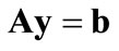 (35)
(35)
 (36)
(36)
where bold face letters signify column vectors for lower case and matrices for upper case letters, y signifies the n-dimensional vector of independent variables, A is an mxn-dimensional vector of parameters, b is an m-dimensional vector of parameters, and k’ is an 1xn-dimensional vector representing the vector transpose of k, and 0 represents the n-dimensional vector with all elements equal to zero. The objective function of Equation (34) is maximized for the standard form.
There are several computationally efficient algorithms that have been developed to solve such linear programming problems in standard form. The original algorithm was developed by George B. Dantzig [2] and it is called the simplex algorithm or the simplex technique. It is based on the premise that the optimal solution for a linear programming problem that maximizes J of Equation (34) is at the vertices of the shape formed by the intersection of the linear equality constraints of Equation (35) that define the feasible region. The simplex algorithm then identifies sequentially non inferior vertex points (vertex points that have an objective value that is higher than previously found) until it finds the maximum solution (optimal solution for the standard form) (for details see [3,4]). It is a computationally efficient algorithm because it takes approximately between m and 2m iterations to arrive at the optimum. Variants of the algorithm suitable for large problems are in use today for implementation in modern day digital computers that are even more efficient (e.g. [5,6]).
For the class of linear programming problems and for each linear programming problem (called the primal in this context), it is possible to formulate its dual programming problem with an optimal solution that matches in value exactly the value of the objective function of the primal at the optimum. The significance of this dual problem is that the optimal solution values of the dual-problem independent variables represent the rates of change of the objective function J with respect to the constraint parameters (elements of vector b). They are typically called shadow prices or marginal values and in several cases have an economic interpretation [7]. For the case of equality constraints, the dual variables are the so-called Lagrange multipliers involved in the solution of constraint optimization problems.
Linear programming formulations and algorithms have been used widely to guide the solution of water allocation and water resources planning problems (e.g. [8]). Their widespread use is a result of the availability of very efficient solvers (as discussed previously) that allow the planner to focus on the problem formulation rather than on the mechanics of the solution algorithm. Some recent examples are mentioned below as illustrations of potential applications. In [9], a series of linear programs are used to solve a water supply problem in Antelope Valley, California, where volumes of water was injected and extracted each year in an unconfined aquifer. In [10], linear programming was used to monitor pollutants and maximize the potable water in a storage reservoir that is used for water delivery via a number of pumping stations. Groundwater management in a saltwater intrusion environment in a coastal karstic aquifer was studied in [11] using linear programming and physical groundwater modeling. In [12] linear programming was used to study conjunctive water use and banking in southern California.
In addition, methods for incorporating uncertainty in problem parameters have been developed that retain the efficiency of solution of the linear programming problems. The basis of these methods is the development of chance constraints where the constraint expresses the probability threshold imposed for the violation of the constraint. Under this constraint formulation and assuming knowledge of the probability distribution of the uncertain parameter, such constraints may be readily converted to ordinary deterministic constraints (e.g. [8,13]).
As an alternative to linear programming problem optimization methods, direct simulation is often used for complex problems. These approaches do not optimize the objective function, but serve as tools to explore various properties of the objective function within the feasible region specified by the constraints. If optimization is necessary for certain system components then simulation is combined with optimization. An example of this approach is the CalSim model used by the US Bureau of Reclamation for reservoir management in California, whereby simulation is coupled with mathematical programming to distribute water volumes throughout the conveyance network of the Central Valley Project of California [14].
Stochastic simulations methods (also referred to as Monte Carlo simulation methods) have also been developed and used to incorporate uncertainty in problem input or problem parameters during the exploration of the properties of the objective function. For instance, a very recent application of Monte Carlo simulation applied stochastic generation techniques to develop risk-based strategies for trading discharge permits in rivers [15]. Also, methods that combine stochastic simulation with systematic optimum search methods have been recently applied to water management problems that involve sequential decisions in the operational management environment (e.g. [16]). The stochastic simulation methods are appropriate when the uncertainty in model parameters can be well characterized through probability distributions (joint probability distributions may be necessary). However, they are computationally expensive and good initial solutions (perhaps obtained by the solution of linear programming problems using the efficient simplex algorithm) are necessary for effective use.
Before we close this short excursion in the literature of mathematical programming for water resources we refer to two additional types of optimization. The first is a recent evolution of mathematical programming called Positive Mathematical Programming [17] and the second is the substantially older and well known class of dynamic programming algorithms [18]. Positive Mathematical Programming is an enhanced mathematical program that includes constraints pertaining to the historical baseline operation of the system to be optimized to include constraints that assure solutions that are similar to system past behavior, and a nonlinear objective function to be optimized for best performance. This type of programming is suitable for analyzing environmental policy when substantial data is available for the calibration process and requires substantial optimization expertise for its solution, as no efficient solvers are currently commercialized. In addition no significant experience exists in introducing uncertainty in model parameters or existing observed data. Dynamic programming is a powerful optimization method suitable for very large problems that involve decisions in stages, with nonlinear objectives and constraints. Well established algorithms exist for stochastic dynamic programming problems with non-negligible uncertainty. There is a long history of the use of dynamic programming in water management with recent applications in participatory decision making for operational water resources management (e.g. [19]). For the application at hand, however, the mathematical program is not large and the linear programming formulation is very efficient so there is no need to introduce dynamic programming as a solution method.
5. Example Programming Problem Solutions
To illustrate the type of solutions that may be obtained from the formulated mathematical program and to demonstrate the feasibility of the formulation, we have constructed a MATLAB sample code that implements a particular version of the formulation using a number of assumed parameters and we perform a small scale sensitivity analysis with respect to demand to illustrate the benefits of such a mathematical programming approach. The mathematical program formulation is solved with a variant of the simplex algorithm implemented in MATLAB. It is noted that the numerical experiments conducted allow for the generation of many possible scenarios of SWP allocations and determine the ensemble of minimum cost solutions as well as certain quantiles of the minimum cost solution ensemble. In all cases, the experiments assume initial condition at the beginning of year 2009, and the planning horizon for the problem is set through year 2013 (5 years).
5.1. Nominal Input and Demand
Table 1 lists the assumed mean annual SWP allocation for each of the years of the planning horizon together with the associated standard deviation of the annual allocation. It is noted that the first year in the planning horizon (Y2009) carries very small uncertainty, because it is assumed that the allocation is already determined when the model is used. The following years carry considerable uncertainty. It is also assumed that dry years will occur in the mean.
Table 2 shows the input parameters used in the numerical experiments. They reflect the information in previous sections and are considered nominal for these numerical experiments.
Figure 1 shows the histogram of the 5-year-average minimum cost from a run that generated 1000 ensemble members (possible SWP allocations). The distribution of minimum average annual costs is approximately Gaussian with a mean of approximately 5.4 million dollars over the planning horizon of 5 years. The minimum costs range from about 5.15 to 5.7 million dollars. No generated sequence of SWP allocations was associated with an infeasible solution.
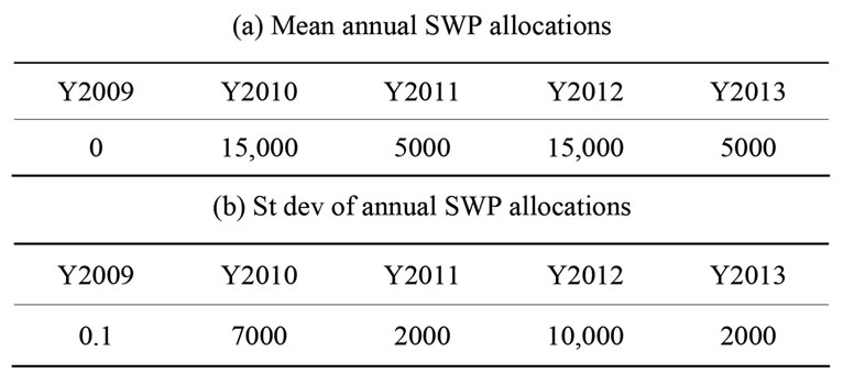
Table 1. Statistics of generated SWP allocations in acre-feet (AF) for CLWA.
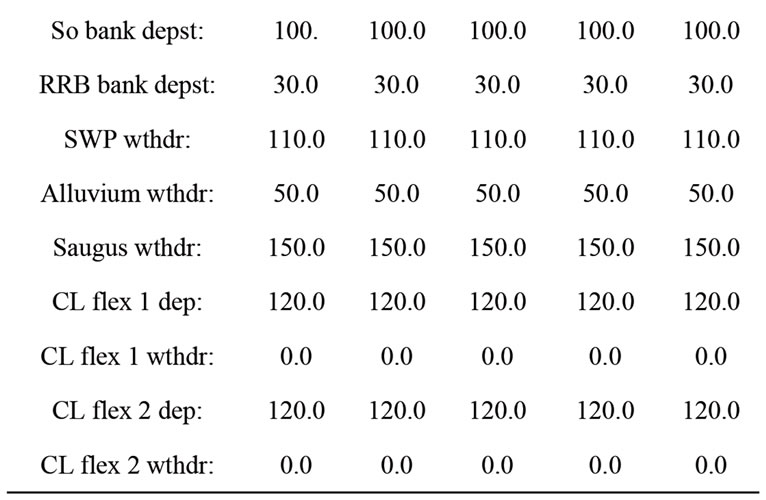
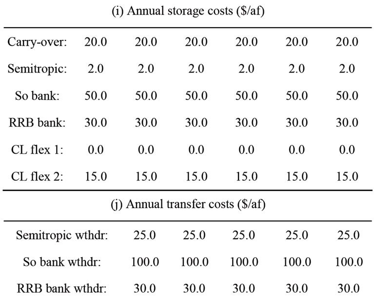
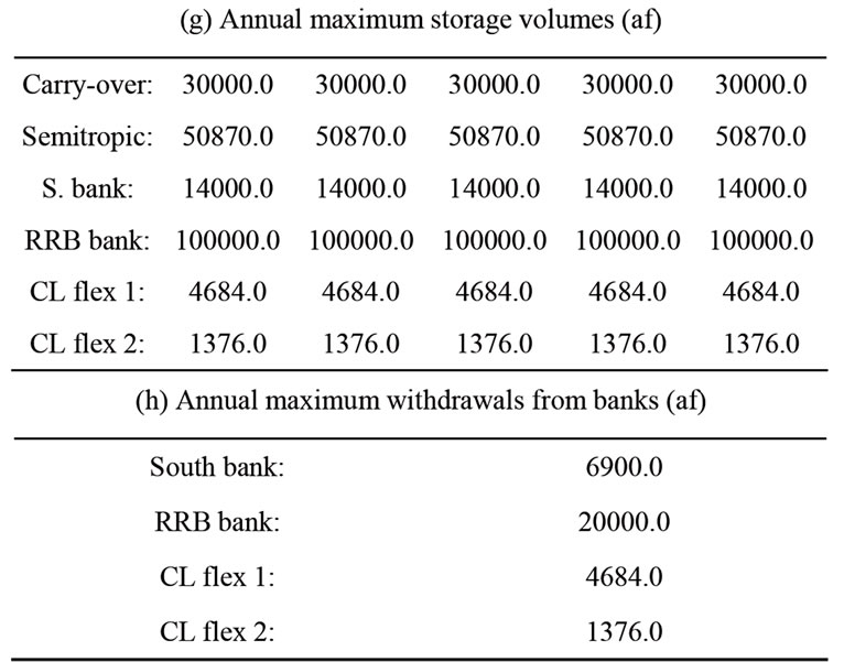
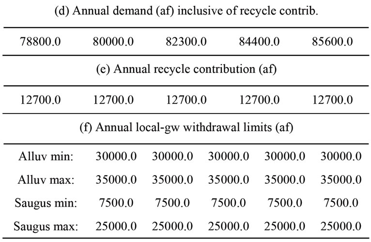
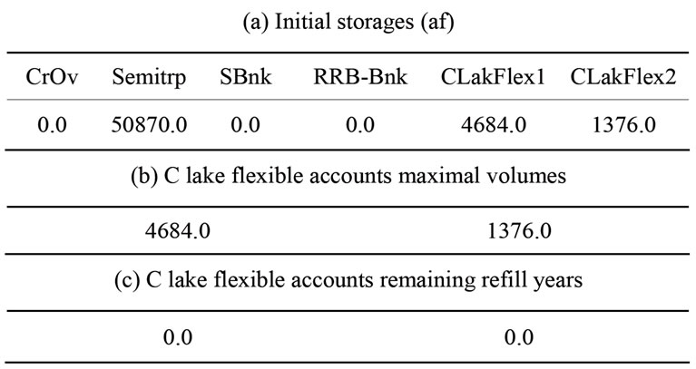
Table 2. Values of initial conditions and input parameters for the 5-year planning horizon.
(i) Annual storage costs ($/af)
(j) Annual transfer costs ($/af)
Figure 1. Histogram of 1000 ensemble members of the 5-year average minimum cost. The cost is in millions of $ per year.
Although the range of 5-year-average minimum costs is considerable, the first year cost for the optimal policies that lead to the minimum 5-year-cost is substantially less dispersed among ensemble members. The reader is reminded that although the solution refers to the optimal policy over the planning horizon of 5 years, only the first year solution may be implemented, using an adaptive principle.
Figure 2 shows the histogram of the first year costs associated with the minimum 5-year-average cost solutions of Figure 1. Very few ensemble members have values different from the bulk of values near 3.6 million per year. In fact, the median and the 95th percentile first year cost are identical for this experiment. Table 3 shows the median first year cost together with the first year solution for the numerical experiment. The allocation of 12,700 af of recycled water is assumed given and it is not considered for the optimization experiment, leaving a total of 66,100 af of first-year demand to be satisfied from various bank and groundwater storages (the first year allocation from SWP is assumed to be 0 af for this experiment). It is shown that the first year demand, assumed to be 78,800 af, is satisfied with a 23,600 af withdrawal from Semitropic bank, a 35,000 af withdrawal from Alluvium groundwater storage, and a 7500 af withdrawal from Saugus groundwater storage. The median first year cost is estimated to be $3587380.0.
The optimal policy for the entire planning horizon for the median first year solution is given in Table 4. Table 4 also shows the generated SWP allocations for this median solution ensemble member. Withdrawals from Semitropic, Alluvium and Saugus formations satisfy the residual annual demands after the recycled water allocation is subtracted from the total annual demand of Table 2 for each year. It is noted that the Semitropic storage is depleted by 2013 as required, and no carryover SWP storage is generated due to the low SWP allocations expected for this experiment. No activity is projected for this solution pertaining to the southern banking storage, the RRB and the Castaic Flexible storages for minimum
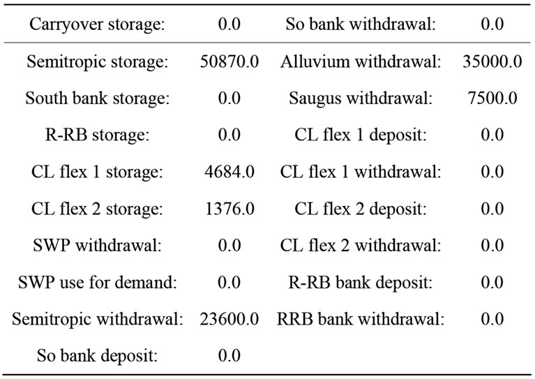
Table 3. Median of first-year cost solutions.
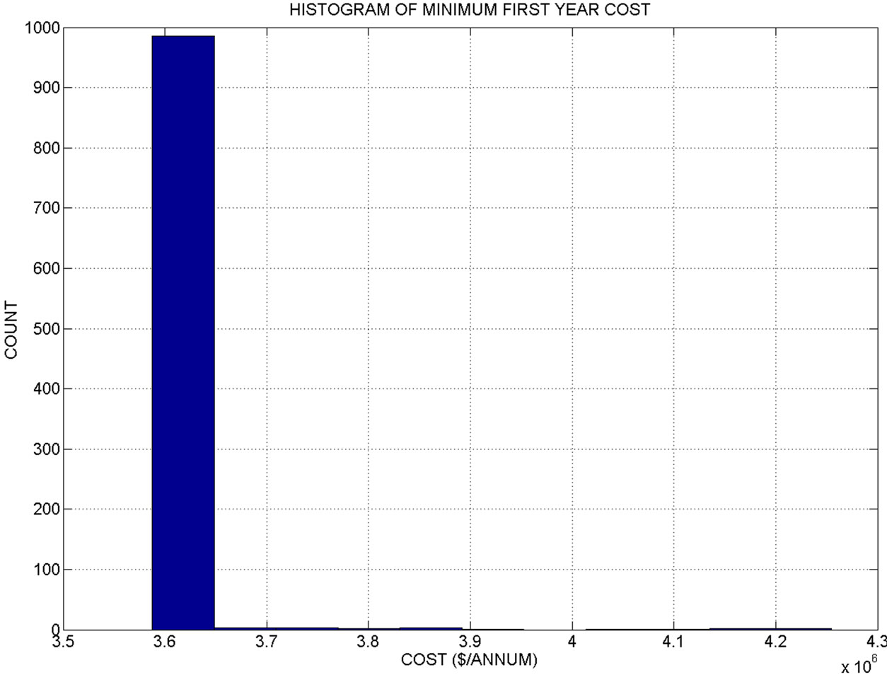
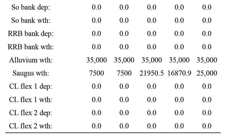
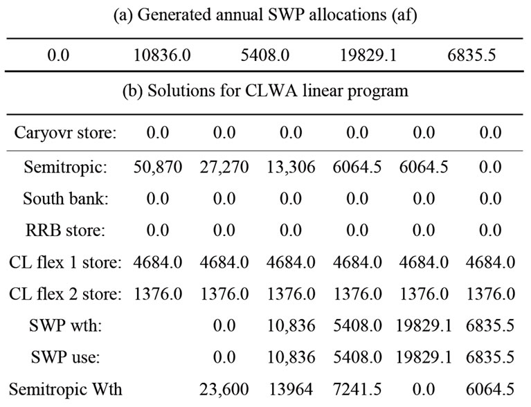
Table 4. Optimal 5-year policy for median of first-year cost solutions.
cost over the 5-year horizon given the SWP allocations generated. The first year total cost is $3587380.0, while the 5-year average annual cost (inclusive of initial storage) is 5379179.2.
5.2. Increasing Demand
In this section we explore the dependence of the optimal solutions to increases in demand. The SWP allocation statistics are as shown in Table 1, and the rest of the input parameters are as shown in Table 2. At first, a 5% increase of demand is imposed for all the years of the 5-year planning horizon. Figure 3 shows the histogram of the 5-year-average minimum costs for 1000 realizations of SWP allocations with the statistics of Table 1.
The Figure shows that the histogram in this case deviates significantly from the Gaussian distribution and it has a median cost that is about 6 million dollars per year; a substantial increase from the 5.4 million dollars per year associated with the nominal solution. That is a 5% increase in demand generates more than a 10% increase in the median 5-year-average minimum cost. The shape of the distribution is truncated for high values of cost due to the fact that there are now realizations of SWP allocations that are infeasible (cannot meet demand due to the violation of the constraint in Equation (32)). In fact, 1.5% of the realizations generated do not have feasible solutions. There is a 1.5% chance that given the statistics of the SWP allocations of Table 1, a 5% increase in demand will not be met.
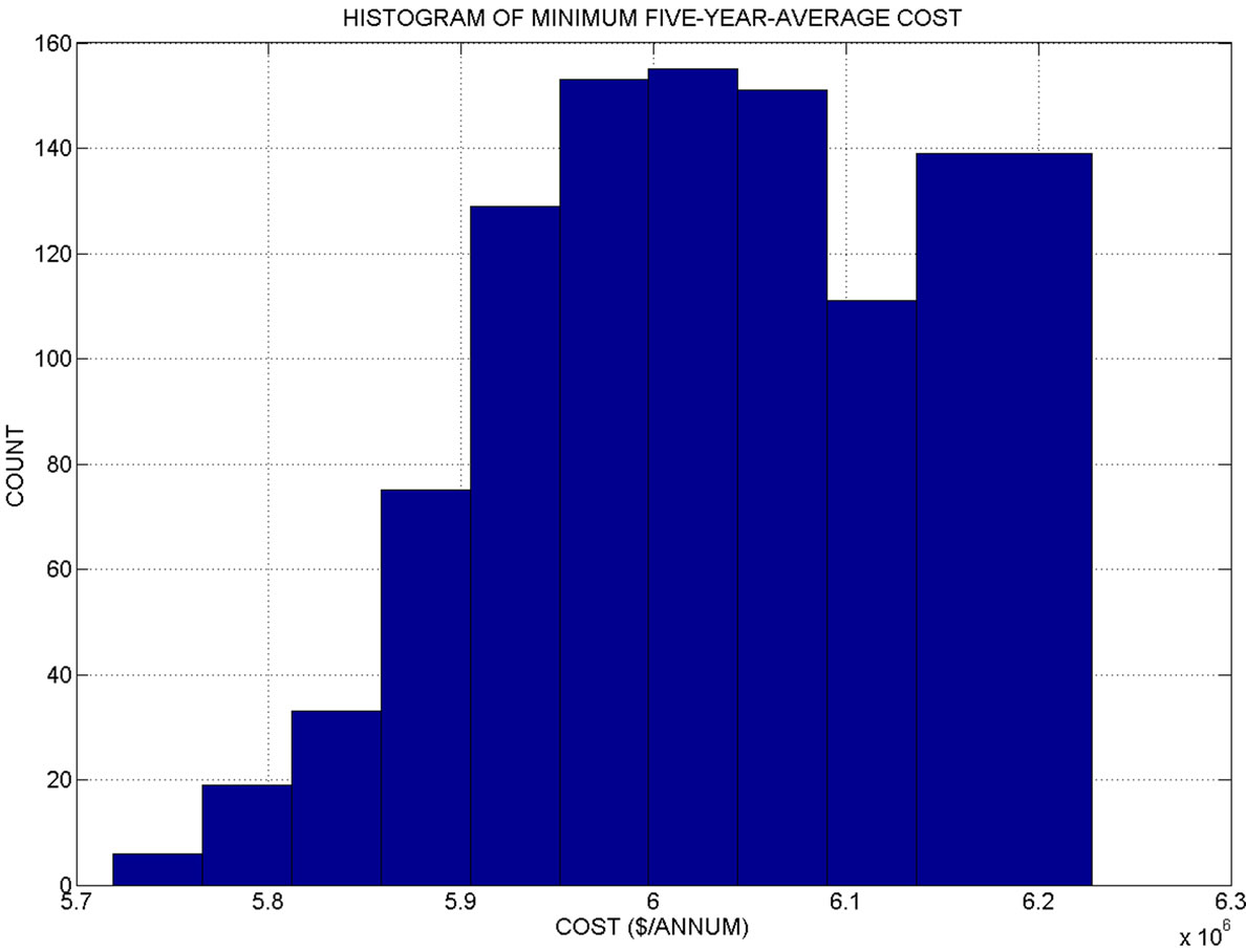
Figure 4 shows the first year cost histogram for the feasible solutions (analogous to Figure 2). Significant increase of the median first-year cost is implied by the long tail of the histogram. The median fist year cost and associated solution are shown in Table 5. The difference in first year median cost from that of the nominal run is due to the increased withdrawal from the Semitropic bank and from the Saugus groundwater formation. The first-year median cost increase is about 5% with respect to the run with nominal demand. This is equal to the 5% increase in demand.
In variance with the nominal case, in this case of increased demand the 95th-percentile first-year cost is different (higher) from the median such cost. Table 5" target="_self"> Table 5 also shows the 95th-percentile cost and associated solution. There is an increase of more than 40% of first year cost with respect to the median first year cost. The demand increase resulted in an increase of first year cost associated with a high probability of meeting demand (risk reduction is in this case associated with substantially increased cost). The cost increase is due to the increase of the withdrawal from the Saugus groundwater storage and a decrease of the Semitropic withdrawal. The full 5-year solutions associated with the median and the 95th-percentile first-year costs discussed above are shown in Tables 6 and 7, respectively. The first year costs are $3780805.0 and $5440467.5, respectively. The 5-year average annual costs are $5964445.0 and $6157747.9, respectively. Different strategies are exhibited over the
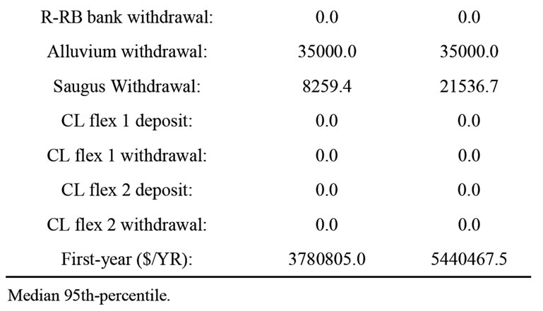
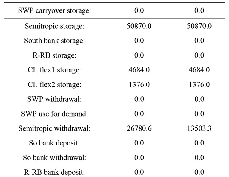
Table 5. Median and 95th-percentile of first-year cost for a demand increase of 5% for all years.
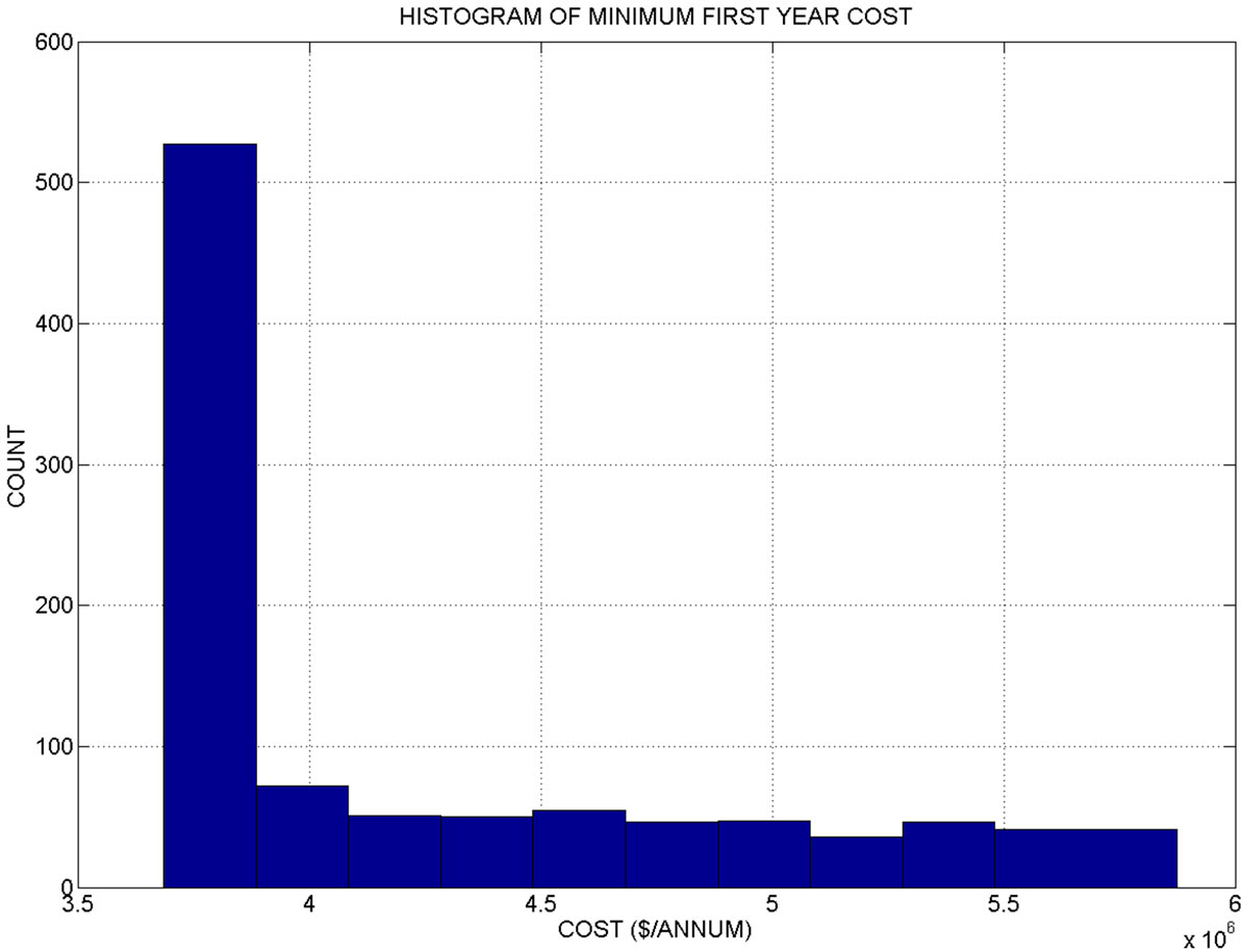
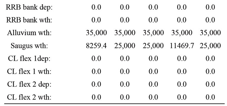
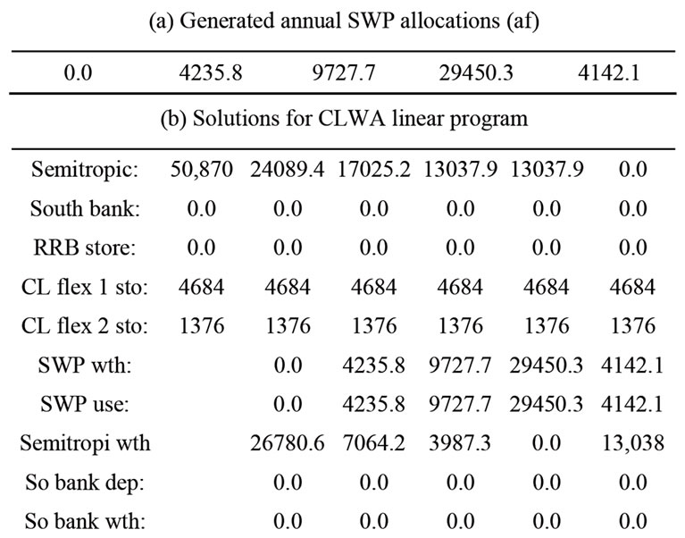
Table 6. Optimal 5-year policy for median of first-year cost solutions for a 5% increase in demand
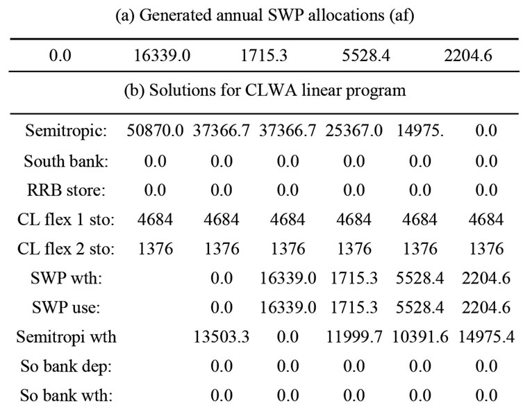
Table 7. Optimal 5-year policy for 95th percentile of first-year cost solutions for a 5% increase in demand.
planning horizon. The SWP allocations are different for the median and the 95th-percentile solutions and this is reflected in the optimal policy for storage and withdrawal. In all cases, the SWP carryover storage remained at zero, and no activity was noted for the southern and RRB banks and the flexible Castaic lake storage.
An additional sensitivity experiment was conducted to determine the variation of the first year cost and of the percent infeasible solutions for a 10% increase of demand for each year of the 5-year planning horizon. The median first-year cost in this case was $5506655.0 and the percent of runs with infeasible solutions rose to 43.4%. It is apparent that a 10% increase of demand under the dry conditions for SWP allocation depicted in the statistics of Table 1 yields a high chance of not being able to meet the demand over the planning horizon. Among the feasible solutions, there is an increase of the median first-year cost of about 54% with respect to the nominal demand run.
The sensitivity of the solution costs to demand changes may be seen in Figure 5. The median first-year cost of the optimal solutions is shown by the bars for increases in demand that span the range from 0 to 10% for each year of the planning horizon. Read on the right vertical axis and indicated by the black heavy line is the corresponding percent of the infeasible solutions (that also describes the risk of failure to meet demand). It is apparent that for the set of assumptions regarding the statistics of the SWP allocation of Table 1 and for the parameters of Table 2 (apart from the demand values), the sensitivity of the median first-year solution with respect to the demand increase as well as the sensitivity of the risk of failure to meet demand increase substantially for percent increases in demand higher than 5%. Up to that value of demand increase, the CLWA system as defined herein exhibits robustness with respect to median first-year cost and risk of failure to meet demand.
6. Concluding Remarks
A linear programming formulation and application is demonstrated for a surfaceand ground-water management problem that involves a variety of water supply sources and the ability for water banking operations. The formulated mathematical optimization problem is designed to minimize the cost of water management operations due to water allocations and water storage over the management horizon of N years with the objective to meet annual water demands.
The mathematical solutions of the resultant minimum cost problem are then used to guide water supply allocation and to study the sensitivity of the minimum cost solutions to water supply uncertainty and to demand increases. The results allow quantitative evaluation of the possible strategies of the water management agency for the first year allocations under the cases examined.
Notable is the significant increase in cost and infeasible solutions with even a moderate increase in water demand. Reliable water demand estimation is then a prerequisite for useful application of the mathematical programming formulations presented to decision making.
REFERENCES
- D. A. Pierre, “Optimization Theory with Applications. Chapter 5,” Dover Publications, Inc., New York, 1986, pp. 193-258.
- G. B. Dantzig, “Maximization of a Linear Function of Variables Subject to Linear Inequalities,” In: T. C. Koopmans, Ed., Activity Analysis of Production and Allocation, Cowles Commission Monograph, No. 13, Wiley, New York, 1951.
- G. B. Dantzig, A. Orden and P. Wolfe, “The Generalized Simplex Method for Minimizing a Linear form under Linear Inequality Constraints,” Pacific Journal of Mathematics, Vol. 5, No. 2, 1955, pp. 183-195.
- G. B. Dantzig, “Linear Programming and Extensions,” Princeton University Press, Princeton, 1963.
- S. Mehrorta, “On the Implementation of a Primal-Dual Interior Point Method,” SIAM Journal on Optimization, Vol. 2, No. 4, 1992, pp. 575-601. doi:10.1137/0802028
- Y. Zhang, “Solving Large-Scale Linear Programs by Interior-Point Methods under the MATLAB Environment,” Technical Report TR96-01, Department of Mathematics and Statistics, University of Maryland, Baltimore, 1995.
- D. M. Simmons, “Nonlinear Programming for Operations Research. Chapter 2,” Prentice-Hall, Inc., Englewood Cliffs, 1975, pp. 26-70.
- D. P. Loucks, J. R. Stedinger and D. A. Haith, “Water Resource Systems Planning and Analysis,” Prentice-Hall, Inc., Englewood Cliffs, 1981.
- D. P. Ahlfeld and G. Baro-Montes, “Solving Unconfined Groundwater Flow Management Problems with Successive Linear Programming,” Journal of Water Resources Planning and Management, Vol. 134, No. 5, 2008, pp. 404-412. doi:10.1061/(ASCE)0733-9496(2008)134:5(404)
- I. Ioslovich and P.-O. Gutman, “Optimal Monitoring and Management of a Water Storage,” Environmental Monitoring and Assessment, Vol. 138, No. 1-2, 2008, pp. 93-100. doi:10.1007/s10661-007-9745-8
- S. M. Kasterakis, G. P. Karatzas, I. K. Nikolos and M. P. Papadopoulou, “Application of Linear Programming and Differential Evolutionary Optimization Methodologies for the Solution of Coastal Subsurface Water Management Problems Subject to Environmental Criteria,” Journal of Hydrology, Vol. 342, No. 3-4, 2007, pp. 270-282.
- M. Pulido-Velazquez, M. W. Jenkins and J. R. Lund “Economic Values for Conjunctive Use and Water Banking in Southern California,” Water Resources Research, Vol. 40, 2004, pp. 1-15. doi:10.1029/2003WR002626
- K. P. Georgakakos and N. E. Graham, “Potential Benefits of Seasonal Inflow Prediction Uncertainty for Reservoir Release Decisions,” Journal of Applied Meteorology and Climatology, Vol. 47, No. 5, 2008, pp. 1297-1321. doi:10.1175/2007JAMC1671.1
- A. J. Draper, A. Munévar, S. K. Arora, E. Reyes, N. L. Parker, F. L. Chung and L. E. Peterson, “CalSim: Generalized Model for Reservoir System Analysis,” Journal of Water Resources Planning and Management, Vol. 130, No. 6, 2004, pp. 480-489. doi:10.1061/(ASCE)0733-9496(2004)130:6(480)
- S. M. Mesbah, R. Kerachian and M. R. Nikoo, “Developing Real Time Operating Rules for Trading Discharge Permits in Rivers: Application of Bayesian Networks,” Environmental Modeling and Software, Vol. 24, No. 2, 2009, pp. 238-246. doi:10.1016/j.envsoft.2008.06.007
- N. E. Graham, K. P. Georgakakos, C. Vargas and M. Echevers, “Simulating the Value of El Nino Forecasts for the Panama Canal,” Advances in Water Resources, Vol. 29, No. 11, 2006, pp. 1667-1677. doi:10.1016/j.advwatres.2005.12.005
- R. E. Howitt, “Positive Mathematical Programming,” American Journal of Agricultural Economics, Vol. 77, No. 2, 1995, pp. 329-342. doi:10.2307/1243543
- R. Bellman, “Dynamic Programming,” Dover Edition 2003, Dover Publications Inc., Mineola, New York, 1972.
- H. Yao and A. Georgakakos, “Assessment of Folsom Lake Response to Historical and Future Climate Scenarios: 2. Reservoir Management,” Journal of Hydrology, Vol. 249, No. 1-4, 2001, pp. 176-196. doi:10.1016/S0022-1694(01)00418-8