Applied Mathematics
Vol. 3 No. 5 (2012) , Article ID: 19057 , 10 pages DOI:10.4236/am.2012.35069
Numerical Approach of Network Problems in Optimal Mass Transportation
1Laboratory of Mathematics of Decision and Numerical Analysis (LMDAN), FASEG, University of Cheikh Anta Diop, Dakar, Senegal
2Unité Mixte Internationale, UMMISCO, Institut de Recherche pour le Développement, Bondy, France
Email: babacar-mbaye.ndiaye@insa-rouen.fr
Received February 13, 2012; revised March 23, 2012; accepted March 31, 2012
Keywords: Optimal Mass Transportation; Network; Urban Traffic; Monge-Kantorovich Problem; Global Optimization
ABSTRACT
In this paper, we focus on the theoretical and numerical aspects of network problems. For an illustration, we consider the urban traffic problems. And our effort is concentrated on the numerical questions to locate the optimal network in a given domain (for example a town). Mainly, our aim is to find the network so as the distance between the population position and the network is minimized. Another problem that we are interested is to give an numerical approach of the Monge and Kantorovitch problems. In the literature, many formulations (see for example [1-4]) have not yet practical applications which deal with the permutation of points. Let us mention interesting numerical works due to E. Oudet begun since at least in 2002. He used genetic algorithms to identify optimal network (see [5]). In this paper we introduce a new reformulation of the problem by introducing permutations . And some examples, based on realistic scenarios, are solved.
1. Introduction
In this paper we present some models of urban planning. These models are examples of applications in mass transportation theory. They describe how to optimize the design of urban structures and their management under realistic assumptions. The paper is organized as follows: in Section 2 we present at first some urban planning models and preliminaries. The Section 3 is devoted to the approximation of the models; and numerical simulations that are our main results. Finally, summary and conclusions are presented in Section 4.
2. Preliminaries and Mathematical Modeling
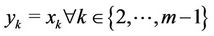
Given two distributions  and
and  on
on  with equal total mass, the classical generic Monge transportation problem consists in finding among all the maps
 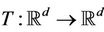 verifying
  for any measurable set in
 , those which solve the minimization problem:
These maps are said to be transportation maps; they transport a measure  (quantity) to a measure
 .
.
For the existence of solutions, we recommend to see [6-10]. We invite the reader to see the books written in this topic by Villani [11,12] for additional information. In particularly Sudakov have studied in [13] the existence of optimal map transportation when  and
and  is absolutely continuous with respect to the Lebesgue measure
 .
.
For studying the many cases where the Monge transportation problem doesn’t give a solution, Kantorovich considered the relaxed version of the Monge problem. In this framework, the transportation problem consists in finding among all admissible measures  having
  and
and  as marginals, those which solve the minimization problem
The meaning of the following expressions  and
and  is explained respectively as follows:
 and
and  for any measurable subset
  of
of .
.
The Monge-Kantorovich problem obtained, depends only on the two distributions  and
and , and the cost
  which may be a function of the path connecting
  to
to .
.
When the unknowns of the problem are the distributions  and
and , the Monge-Kantorovich mass transportation problemcan be interpreted as an optimal urban design problem. When the unknown is the transportation network, we have an irrigation problem, that is an optimal design of public transportation networks.
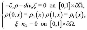
We also mention the dynamic formulation of mass transportation given in [4,14,15] and generalized in [16]. In this framework, we consider that:
· the space of measures acting is a time-space domain  where the urban area
  is a bounded Lipschitz open subset with outward normal vector
 ;
;
· the mass density  at the position
  and time
  is a Borel measure supported on
 , i.e.
 ;
;
· the velocity field  of a particle at
  is a Borel vectorial measures supported on
 ;
;
· the velocity field  of the flow at
  is a Borel vectorial measures supported on

 and defined by
  .
.
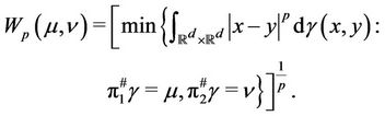
The Monge-Kantorovich mass transportation problem consists in solving the following optimization problem:
 (1)
(1)
with the constraints:
 (2)
(2)
where  is an integral functional on the
  -valued measures defined on
 . Note that (2) is the continuity equation of our mass transportation model.
2.1. Optimal Urban Design
In the models of optimal design of an urban area we considered that
· the urban area  is a well known regular compact subset of
 ;
;
· the total population and the total production are fixed data of the problem;
· only the density of residents  and the density of services
  are unknowns data of the problem.
The aim is to find the density of residents  and the density of services
  minimizing the transportation cost.
Principally there are two models for studying the optimal urban design. The first one takes into account the following facts:
· there is a transportation cost for moving from the residential areas to the services poles;
· people do not desire to live in areas where the density of population is too high;
· services need to be concentrated as much as possible, in order to increase efficiency and decrease management costs.
The transportation cost will be described through a Monge-Kantorovich mass transportation model.
In particularly, we will take it as the  -Wasserstein distance defined by:
Taking into account the total unhappiness of residents due to high density of population, we define a penalization functional of the form

where  is the density of the population,
  is supposed to be convex, null at the origin and super linear (that is
  as
as ). The increasing and diverging function
  represents the unhappiness to live in an area with population density
 .
.
Thus we define a functional  which penalizes sparse services. This functional is of the form:
where  is supposed to be concavenull with infinite slope at the origin (i.e.
  as
as  ). Every single term
  in the sum above represents the cost for building and managing a service pole of size
  located at the point
  of
of . The Report
  is the productivity of pole of size
 .
.
So in the first model, the optimal urban design problem becomes the following optimization problem:
 (3)
(3)
In the second model the population transportation is considered as a flow, that is a vector field . The equilibrium condition is achieved when the emerging flow is the excess of the demand in
 , i.e.

In order to take into account the congestion effects, we suppose that the transportation cost  per resident at the point
  depends on the traffic intensity at
 , i.e.
where  is an increasing function.
Then, the transportation cost moving  to
to  is:
is:
The problem (1) with the constraints (2) allows both to take into account the congestion effects by an appropriated choice of the functionals  and to widen the choice of unhappiness function
  and management cost function
  of the first model to the local lower semicontinuous functionals on
 .
.
For more details, we refer the interested reader to the several recent papers on the subject (see for instance [4, 14-17]).
2.2. Network Problems Applied to the Urban Transportation
In the models of optimal design of an urban area we considered that
· the urban area  is a well known regular compact subset of
 ;
;
· the density of residents  and the density of services
  are two well known positives measures with equal mass.
The irrigation problem consists to find among all feasible structures (or feasible network)  those that minimize the transportation cost
The particular irrigation problem of the average distance consists to find an optimal network  for which the average distance for a citizen to reach the mos
  t nearby point of the network is minimal.

Theorem 1 For every  there exists an optimal network
  for the Optimization problem

where  is the Hausdorff measure defined on
 .
.
Notice that there are other proposition of functionals to be minimized.
For more details, we refer the interested reader to the several recent papers on the subject (see for instance [1-3, 18,19]).
Our aim is to concentrate our effort on the numerical questions to locate the optimal network in a given domain  says for example a town.
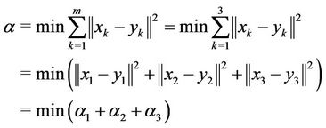
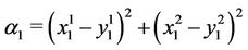
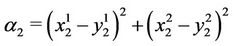
3. Approximation and Numerical Simulations
3.1. First Steps for the Formulation of the Discrete Problem
In this subsection, we are going to propose a first approach of discretization. From this, we deduce a generalized formulation but not the own possible formulation.
Let

For the simulation we are going to consider:
·  and
and ;
;
·  such that
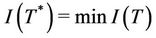 ;
;
· a sequence of points  and of balls
  such that
 , with
 , and
, and .
.
and let  and
and . We build an other map
  switching round cyclically the images of balls
 . Then
  satisfies
where  and
and .
.
Then we have , i.e.
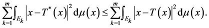
Therefore when , we obtain
 (4)
(4)
Suppose that the map  and the measure
  are regular, the Equation (4) leads
 (5)
(5)
Then 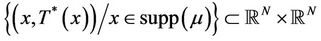
is cyclically monotonous and .
.
At first, in problem ( ) the objective is to find the points
  which minimize
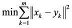 subject to
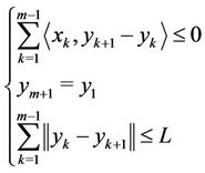
In the next section, we show that it is quite possible to give a more general approximation .
3.2. New Reformulation Using Permutations
In the literature, many formulations (see for example [1-4]) have not yet practical applications which deal with the permutation of points. In this paper we introduce a new reformulation of the problem by introducing permutations .
.
Let us take a permutation  defined on
  such that
 , we set:
and we solve the two following problems: ( )
)

subject to

and problem ( )
)
subject to
with the norm  and
and
 .
.
This is a theoretical formulation. And our aim is to apply it to a practical urban transport network. As a first step, we decided to work on  with a reasonable number of points.
For a scenario in , if we consider
  points: the number of programs to be solved becomes
 . We leave the reader to verify that for:
· m = 3 points  we solve 27 programs
· m = 4 points  we solve 256 programs
· etc.
A scenario involving up to 18 points is used for problem ( ). Using this scenario with problems (
 ) and (
 ) requires to solve
  programs, it is the reason we consider only some of these points for permutations in (
 ) and (
 ).
).
3.3. Numerical Experiments
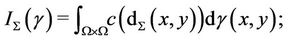
This section shows how the three models developed in the two previous Sections 3.1 and 3.2 are applied to real data of Dakar Dem Dikk (3D). Recall that 3D (see [20], [21]) is the main public urban transportation company in Dakar. This company manages a fleet of buses with different technical characteristics. Some of the buses can operate only in certain roads in the city center and the others can access in all over the network. Buses are parked overnight at Ouakam and Thiaroye terminals (see Figure 1).
To ensure network coverage, 3D manages its services by using 17 lines, with 11 from Ouakam terminal and 6 from Thiaroye terminal. Each line ensures a certain num-
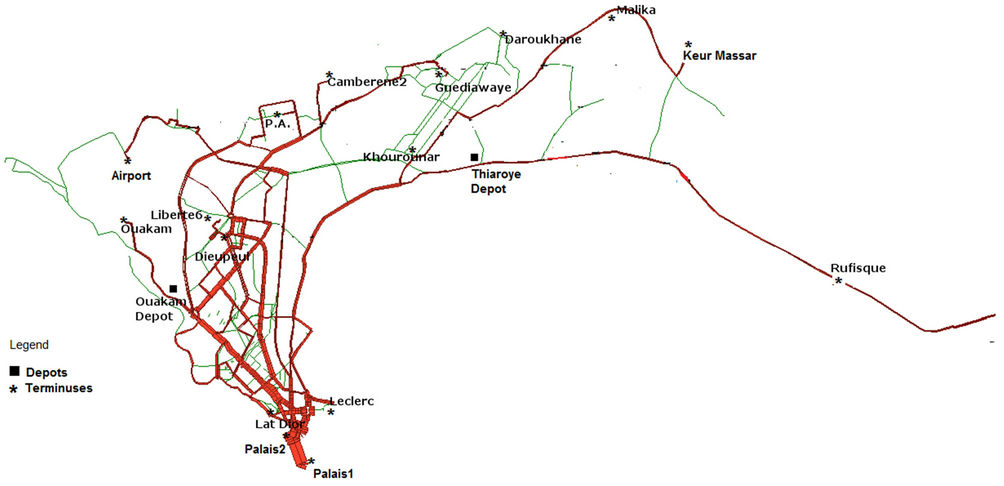
Figure 1. Urban transportation network of 3D.
ber of routes. At present, the total number of routes in the network is 289. First, the most important 18 sites of the network are identified. Thirty (30) permanent terminuses (terminals) and 810 bus stops are used (see Figure 1, where bus stops are not represented due to their size). The map in Figure 1 is obtained by using the software EMME [22]. Table 1 gives the 18 sites, their latitude and longitude.
The data are based on the scenario of 3D; and the input data needed to use the models are the:
· total length of the network  kilometers;
· number of points  (terminals and bus stops)
  (see Figure 1);
· latitude and longitude of points  representing the two terminals and bus stops.
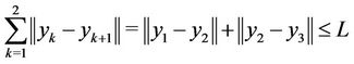
The total distance covered by all the buses from terminals to starting points of routes and from end points back to their terminals represents the total length of the network; and we have L = 5902.62 kilometers (for the 18 sites).
The GPS (Global Positioning System) coordinates are calculated with Google map, and then transformed into coordinates on the plane with he formula: degree + (minute/60) + (second/3600). Table 1 gives the coordinates of all points.
The numerical experiments are executed:
· on a computer: 2 × Intel(R) Core(TM)2 Duo CPU 2.00 GHz, 4.0 Gb of RAM, under UNIX system;
· and by the software IPOPT (Interior Point OPTimization) 3.9 stable [23,24], running with linear solver ma27.
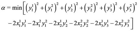
For the objective function, we have:
with
Finally,
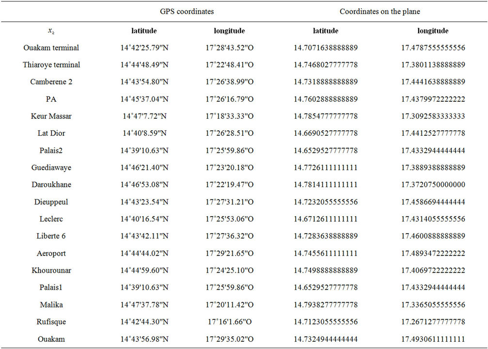
Table 1. Scenario of 3D.
and 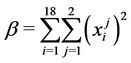 is added to the value of the objective function.
Constraint  gives
gives
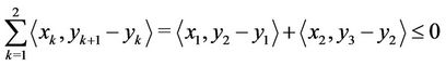 .
.
Urban transportation network of 3D Thus, 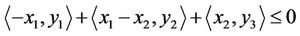 , i.e.:

And  gives
gives
 i.e.:
i.e.:
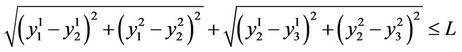
with  and
and .
.
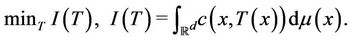
We simply formulate the problem in AMPL [25] syntax, and solve the problem through the AMPL environment; with a total number of 38 variables for problem . The solution obtained is an optimal one (for each case) wherein the priority is assigned to the minimization of the distance between
  and
and . The IPOPT found an optimal point within desired tolerances; and we obtain the following results: the total number of iterations is 16 and for the optimal network
  we have
 . The others obtained solutions
 ,
,  and
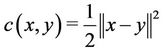
and  are given in Table 2 with the GPS coordinates. The points
  and
and  are represented in the network (see Figure 2).
Permutations make the resolution more complicated but can give better results. The number of sub-problems to solve depends on the number of points in the network. Thus, we choose  points in 3D’s network.
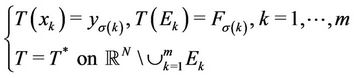
Now, let us take the permutation which is the main idea of this work. For problem ,
,  such that
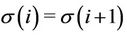 , we have
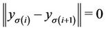 . Therefore some constraints are similar and we have 9 subproblems to solve. An illustration:

The three unconstrained sub-problems are obtained for  with
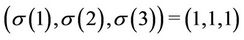
with , i.e. in the three permutations (1,1,1), (2,2,2) and (3,3,3).
All sub-problems constraints are reported in Table 3.
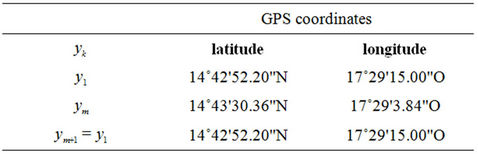
Table 2. y1 and ym for optimal network Σopt.

Figure 2. Optimal network of 3D without permutation.
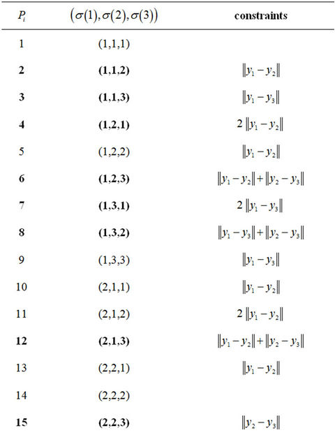
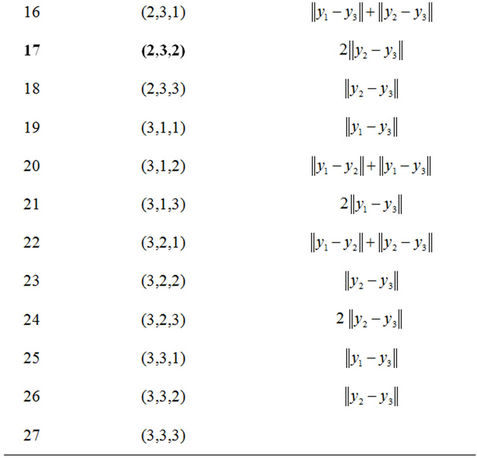
Table 3. All constraints with permutations.
It is sufficient to solve 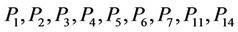 and
and ; since we have
 ,
,  ,
, 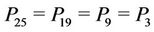 ,
,  ,
,  ,
,  ,
,  ,
,  ,
,  and
and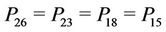 .
.
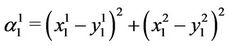
We only compute the quantities ,
,  and
and . For all sub-problems
 , the objective function is the same as problem
  with
with .
.
with
 ,
,
and
 .
.
Finally,
and  is added to the value of the objective function.
From computational results, we have obtained the same value for all 10 sub-problems. Thus, permutations do not influence the distance constraint on the curve of . The optimal value is
  for all
  with
with .
.
For problem , we consider
  and the number of possible permutation is
 . Recall that the number of sub-problems to solve depends on the number of points in the network. Also, we choose
  points in 3D’s network. Thus, for the considered permutation
  we have obtained a total of
  sub-problems
  to solve, see Table 4.
In order not to overload explanations, we develop only the sub-problem , the rest are left to the reader as an exercise.
In , the sub-problem
  is obtained for
 with vectors
  and
and 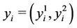
 . For the objective function, we have

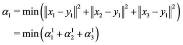
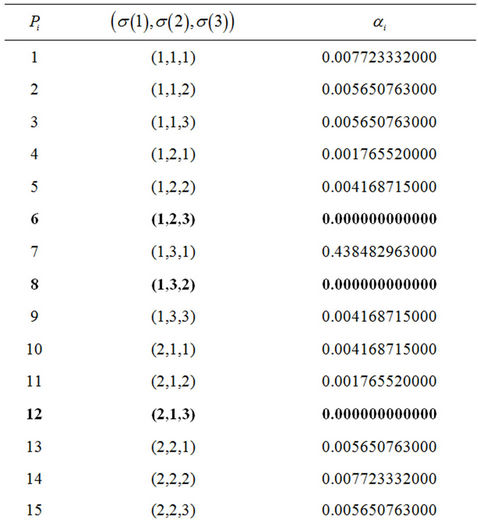

Table 4. Optimal values of αi with different permutations.
with
 ,
,
and

Finally,
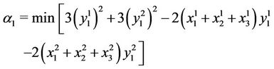
and 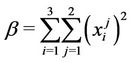 is added to the value of the objective function for all sub-problems
The constraint

gives
 i.e.:
i.e.:

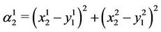
For the scenario of problems  and
and , we choose x1 = Ouakam terminal, x2 = Thiaroye terminal and x3 = Leclerc (see Table 5).
We denote by  and
and  the optimal value and the optimal solution of sub-problem
 , respectively.
The results show that the following six sub-problems: ,
,  ,
,  ,
,  ,
,  ,
,  give the best value
  . The six solutions are different, i.e.:
 with only
 .
.
The curve  can be described by one of the points
 ; see Figure 3 where
 .
.
The points  which define
  (with coordinates
 are given in Table 6, with
 .
.
The solutions giving the best possible permutations (optimum) are illustrated in Table 6 and include all permutations .
.
According to the simulations, we determine a set of optimal policy that can describe the optimal network . Finally: after comparison of the simulated models, we can deduce that the model for problem
  is better. It provides the best curve describing the optimal value
 , obtained with the permutations introduced in the objective function.
4. Conclusions
In this paper, we describe applications of mass transportation theory and develop how to optimize the curve design of urban network problems. Using the discrete formulations, we give three nonlinear programming problems with continue variables, and have described urban transportation problem of 3D applied to these three models. The results have shown that the optimal network is obtained with permutations including .
.
In future works, we will study an application in  and make a reformulation that solves a unique program,
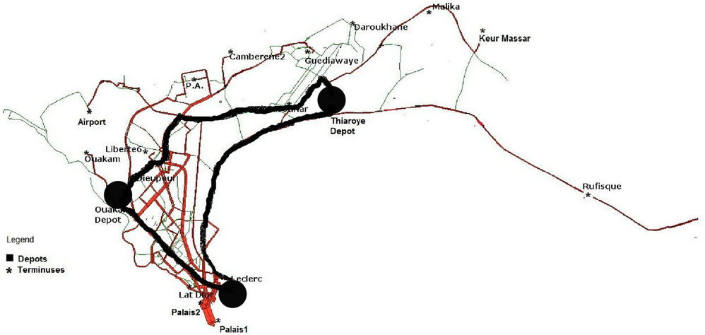
Figure 3. Optimal network Σopt.

Table 5. The network Σopt with permutations.
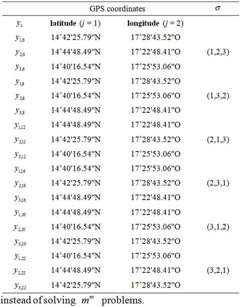
Table 6. The optimal solutions  with permutations.
5. Acknowledgements
We would like to thank all DSI’s (Division Système d’Information) members of 3D for their time and efforts for providing the data, and discussions related to the meaning of the data.
REFERENCES
- A. Figalli, “Optimal Transportation and Action-Minimizing Measures,” Ph.D. Thesis, Scuola Normale Superiore, Pisa, 2007.
- G. Buttazzo, E. Oudet and E. Stepanov, “Optimal Transportation Problems with Free Dirichlet Regions,” Progress in Non-Linear Differential Equations, Vol. 51, 2002, pp. 41-65.
- G. Buttazzo, A. Pratelli, S. Solimini and E. Stepanov, “Optimal Urbain Networks via Mass Transportation,” Lecture Notes in Mathematics, Vol. 1961, 2009, pp. 75- 103.
- G. Buttazzo, “Three Optimization Problems in Mass Transportation Theory,” Nonsmooth Mechanics and Analysis, Vol. 12, 2006, pp. 13-23.
- E. Oudet, “Some Results in Shape Optimization and Optimization,” 2002. http://www-ljk.imag.fr/membres/Edouard.Oudet/index.php?page=cv/node2
- L. Ambrosio, “Mathematical Aspects of Evolving Interfaces,” Lectures Notes in Mathematics, Vol. 1812, 2003, pp. 1-52.
- L. Ambrosio and P. Tilli, “Select Topics on ‘Analysis on Metric Espaces’,” Appunti dei Corsi Tenuti da Docenti delle Scuola, Scuola Normale superiore, Pisa, 2000.
- L. Caffarelli, M. Feldman and R. J. McCann, “Constructing Optimal Maps for Monge’s Transport Problem as a Limit of Strictly Convex Costs,” Journal of the American Mathematical Society, Vol. 15, No. 1, 2002, pp. 1-26. doi:10.1090/S0894-0347-01-00376-9
- L. C. Evans and W. Gangbo, “Differential Equations Methods for the Monge-Kantorovich Mass Transfer Problem,” Memoirs of the American Mathematical Society, Vol. 137, No. 653, 1999, pp. 1-66.
- A. Pratelli, “Existence of Optimal Transport Maps and Regularity of the Transport Density in Masse Transportation Problems,” Ph.D. Thesis, Scuola Normale Superiore, Pisa, 2003. http://cvgmt.sns.it/
- C. Villani, “Topics in Optimal Transportation,” Graduate Studies in Mathematics, Vol. 58, 2003.
- C. Villani, “Optimal Transport, Old and New,” Springer, Berlin, 2008.
- V. N. Sudakov, “Geometric Problems in the Theory of Infinite Dimensional Distributions,” Proceedings of the Steklov Institute of Mathematics, Vol. 141, 1976, pp. 1- 178.
- Y. Brenier, “Optimal Transportation and Applications,” Extended Monge-Kantorovich Theory,” Lecture Notes in Mathematics, Vol. 1813, 2003, pp. 91-121.
- G. Carlier, C. Jimenez and F. Santambrogio, “Optimal Transportation with Traffic Congestion and Wardrop Equilibria,” CVGMT Prepint, 2006. http://cvgmt.sns.it
- G. Buttazzo, C. Jimenez and E. Oudet, “An Optimization Problem for Mass Transportation with Congested Dynamics,” SIAM Journal on Control and Optimization, Vol. 48, No. 3, 2009.
- F. Santambrogio, “Variational Problems in Transport Theory with Mass Concentration,” Ph.D. Thesis, Scuola Normale Superiore, 2006.
- A. Brancolini and G. Buttazzo, “Optimal Networks for Mass Transportation Problems,” Preprint Diparttimento di Matematica Universit di Pisa, Pisa, 2003.
- G. Buttazzo and E. Stepanov, “Optimal Transportation Networks as Free Dirichlet Regions for the Monge-Kantorovich Problem,” Annali della Scuola Normale Superiore di Pisa—Classe di Scienze, Vol. 2, No. 4, 2003, pp. 631-678.
- C. B. Djiba, “Optimal Assignment of Routes to a Terminal for an Urban Transport Network,” Master of Research Engineering Sciences, Cheikh Anta Diop University, ESP Dakar, 2008.
- Dakar Dem Dikk, Full Traffic 2008-2009, File InputOutput, 2008. http://www.demdikk.com
- INRO Consultants Inc., “EMME User’s Manual,” 2007.
- A. Wächter and L. T. Biegler, “Line Search Filter Methods for Nonlinear Programming: Motivation and Global Convergence,” SIAM Journal on Optimization, Vol. 16, No. 1, 2005, pp. 1-31. doi:10.1137/S1052623403426556
- A. Wächter and L. T. Biegler, “On the Implementation of a Primal-Dual Interior Point Filter Line Search Algorithm for Large-Scale Nonlinear Programming,” Mathematical Programming, Vol. 106, No. 1, 2006, pp. 25-57. doi:10.1007/s10107-004-0559-y
- R. Fourer, D. M. Gay and B. W. Kernighan, “AMPL: A Modeling Language For Mathematical Programming,” Thomson Publishing Company, Danvers, 1993.