ABSTRACT

Asset pricing under the certainty equivalent approach framework always raises the current value of the asset with the riskless rate first, followed immediately by risk adjustments. Clearly, this type of arrangement does not apply to assets that are expecting to lose values if it were to adhere to feasible economic reasoning. By using the put-call parity relationship and its underlying law of no arbitrage, the needed expected rates of return for the job of option pricing can thus be obtained. This study suggests a new model in old fashion, which can better satisfy the empirical criticism of the Black-Scholes option pricing model.

1. Introduction

Standard financial textbooks recommend two basic approaches to capital budgeting. The first is to calculate the expected value of a project, and then to adopt an uncertain discount rate to obtain the present value of the project. In most occasions, this is called the net present value (NPV) with uncertainty approach. In contrast, the second approach is used to transform the expected value of the project immediately into a certainty equivalent value that is free of any uncertainties, and then to directly apply the riskless discount rate from the market to obtain the present value of the project. Similarly well known as the first approach, this has been termed the certainty equivalent (CEQ) approach. The problem with the latter approach is that its logic of calculation does not conform to overall economic reasoning; hence, its feasibility to price options is questionable. Nevertheless, the traditional NPV approach still has its own deficiency in the management of option pricing. Usually uncertain discount rates must be created in a normative instead of a positive manner (Yu, 2012) [1], and they are certainly not perfectly applicable to price options, which can consequently have direct connections with their underlying assets in returns and risks. Furthermore, if a unique way of determining the needed uncertain discount rates in the positive sense exits, applying uncertain discount rates in the normative sense for option pricing must then become unacceptable.

Traditionally, the law of no arbitrage is the mainstream concept for price options. Irrespective of whether it is the Black and Scholes (1973) [2] option pricing model (BSOPM) or a similar product such as the binomial model by Cox et al. (1979) [3], “(T)he underlying idea is that an investor could exactly replicate the payoff of the option by trading at each point in time in the stock and a riskless bond∙∙∙ For the market to be free from arbitrage opportunities, the cost of the replicating strategy must be the exact price of the option” (Dimson & Mussarian, 1999, p. 1761) [4]. However, because the method to constructing the hedging portfolio is itself consistent with the framework of the CEQ approach, it may be unavoidable to only have mathematical feasibility but no economic feasibility.

This study has three main tasks. First, we explain why the BSOPM is conducted by following the framework of the CEQ approach which, in turn, has a difficulty to address economic feasibility. Second, we demonstrate how to employ the law of no arbitrage to acquire the needed uncertain discount rates for option pricing under the NPV approach. Finally, we provide simple simulation tests to further verify the economic feasibility of the suggested option pricing model.

2. The CEQ Approach

The entire process of deriving the BSOPM can generally be divided into the following two stages: In the first, the main task is to establish a riskless discount rate and create a form of heat equation in physics; in the second, the main task is to determine the effective range of values of the option, to adopt the Fourier integral technique to solve the expected value of the option. All related details of derivation can be found in the Kutner (1988) [5] study. A careful examination showed that this framework of two-stage derivation can be demonstrated exactly under the CEQ approach.

Taking a call as an example, after setting the price of its underlying asset at the maturity date T as and its exercise price as X, its terminal value can then be stated as. According to the NPV approachthe current price of this call C₀ must be exactly equal to the discounted expected value of this terminal value, and can be expressed mathematically as

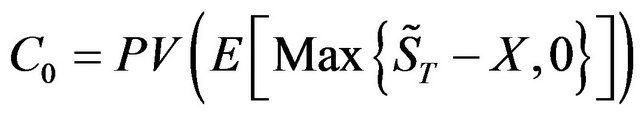(1)

This equation can be re-written in more detail as

(2)

Under the assumptions of the BSOPM, the connection between and its present price S₀ can be listed as

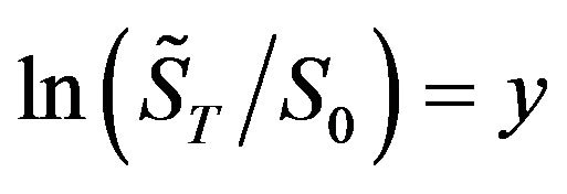(3)

Hence, it can be further re-arranged into

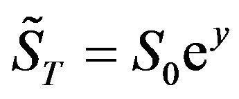(4)

By following the CEQ approach, with Equation (4) and the riskless discount factor, Equation (2) can be transformed into

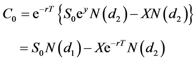(5)

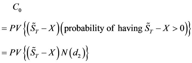
The whole process is thus far exactly the same as the outline of the first BSOPM stage of deriving the call. Consequently, the main aim in the second stage of the model is to solve the cumulative probability factor, to verify the expected value listed in Equation (2). The peculiar thing about this stage is that everything must occur instantaneously.

The framework of the CEQ approach is also evidently applicable to the Cox et al. (1979) [3] binomial model, as can be further explained in the followings: For only a short period t after limiting the terminal price of the underlying asset to only two possible outcomes of S_u and S_d, the corresponding terminal values for either call or put is a set of C_u and C_d or of P_u and P_d, respectively. After constructing a hedging portfolio consisting of the underlying asset plus cash and having the same random payoff as the call (or put), the current price of the call can thus be

(6)

in which, π is the so-called risk-neutral probability, and the price for the corresponding put is

(7)

With an exercise price X, all four possible terminal values for both call and put can be entered into Equations (6) and (7) first, before replacing the left-hand side of the following put-call parity relationship

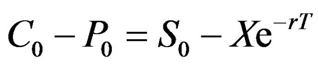(8)

Finally, regardless of what may occur to all of these four possible terminal values, the following outcome is always concluded as

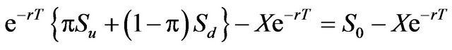(9)

For the underlying asset, its current price S₀ can now be clearly determined directly based on the framework of the CEQ approach. In other words, within the binomial approach, the method for constructing the hedging portfolio from the beginning must follow the logic behind the first stage of the CEQ approach.

However, under the assumption of Ceteris Paribus, future movements can never be advantageous to both call and put. This means that, although inflating the current price with a riskless rate for either call or put is mathematically permissible, it is still impossible to interpret the calculated outcome with any acceptable economic reasoning. When terminal conditions for both call and put must be expressed in the opposite manner, the corresponding expectation of future values for either party goes against each other. In other words, under no circumstances can simultaneously inflating the current prices of both call and put with a riskless rate be consistent with the relationship between those two terminal call and put values. Moreover, in our financial market, it is common to find the future price of an asset to be lower than its spot price.

The disclaimer of the BSOPM is that it exists in a world of risk neutrality, and the expected rate of return of its underlying asset can thus be totally discarded. However, “(E)ven Black and Scholes found it hard to provide a good intuition for this result” (Dimson & Mussarian, 1999, p. 1761) [4]. Moreover, because the expected rate of return for a newly-existent option is not directly observable, it is reasonable to consider switching from the NPV to the CEQ approach to circumvent this difficulty. However, because the latter cannot be economically feasible, returning to the former remains the only choice. Based on this rationale, a different idea of determining the needed uncertain expected rates of return for option pricing under the NPV approach must be considered.

3. Pricing European Options under the Law of No Arbitrage

To re-examine Equation (1) describing the pricing of a European call, because its effective value is confined within the range where is greater than, the expected terminal value of this call can be stated as

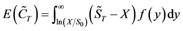(10)

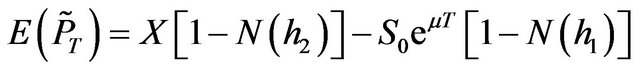
and the expected terminal value of the corresponding put as

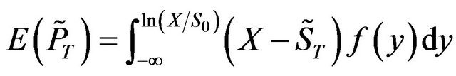(11)

Under the framework of the NPV approach, Smith, Jr. (1976) [6] clearly demonstrated that Equation (10) can be expressed in details as

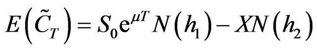(12)

in which, μ is the expected rate of return for the underlying asset of the call, and

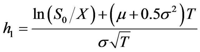(13a)

(13b)

Similarly, Equation (11) can be listed as

(14)

In addition, expected rates of return for both call and put can be expressed directly as

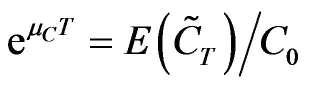(15)

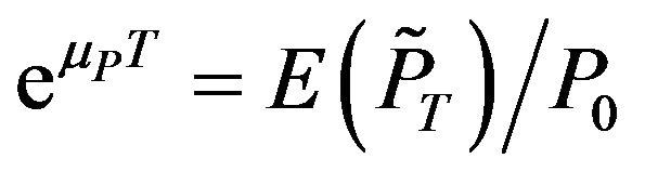(16)

After substituting Equations (12) to (16) into Equation (8), which represents the put-call parity relationship, the outcome becomes

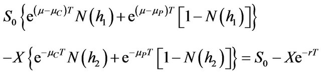(17)

Under the law of no arbitrage, the following two relationships must thus hold

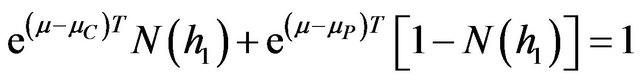(18)

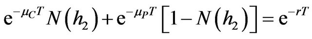(19)

The expected rates of return for both call and put can now be calculated separately as

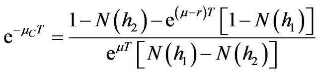(20a)

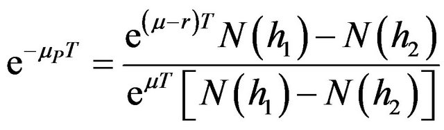(20b)

Finally, current prices for both call and put can be presented as

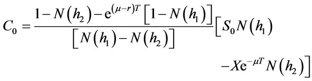(21)

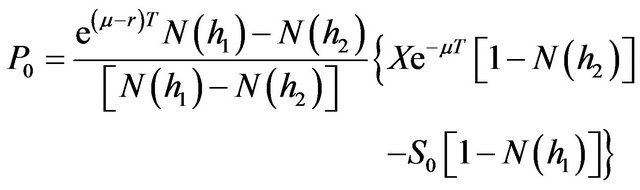(22)

Clearly, if the expected rate of return of the underlying asset μ is exactly equal to the riskless rate, then both Equations (21) and (22) conform to the BSOPM. Furthermore, both equations have a natural limitation; that is, and cannot be equal or close to 1, which means that the possibility of success is one hundred percent or near. If this were the case, then the whole pricing job would have to be re-adjusted to address a riskless condition.

4. Simulation Tests

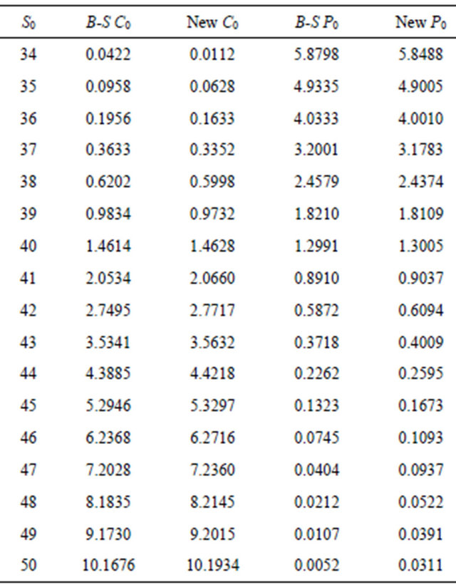
Other than the necessary condition of conforming to the put-call parity relationship presented in Equation (8), more pieces of evidence should also be provided to further support the feasibility of Equations (21) and (22). Simulation results for both the BSOPM and suggested models are listed in Table 1 after we arbitrarily set the exercise price X at 40, the expected rate of return μ at 0.12 and its corresponding standard deviation σ for the underlying asset at 0.03, the annual riskless rate r at 0.0488 and the maturity date T at 0.0833 year. Based on major findings in past empirical studies on the BSOPM such as the one conducted by MacBeth and Merville (1979) [7], this clearly indicated that on average the pricing outcome for in-(or out-)the-money Black-Scholes call is lower (or higher) than the actual market price; the more out of the money, the more significant the pricing bias. Regarding put, the criticism is exactly opposite. Table 1 shows that the suggested models can better satisfy all criticisms. However, whereas absolute deviations are not significantly large, this may explain why the BSOPM remains the most widely-adopted model for pricing European options to date.

Table 1. Pricing outcomes simulated from different models.

5. Conclusions

A Comparing of the BSOPM and the model proposed from this study shows that one of the main differences is the inclusion of information regarding the expected rate of return for the underlying asset of the option in the proposed model. According to the simple rules of dominance, when the risk measures are equivalent for two different assets, whichever has the higher expected rate of return should thus have a better evaluation, and hence, a higher market value. Disregarding this point certainly violates the principle of informational efficiency in the financial market. This may be the reason the BSOPM remains applicable when the expected rate of return for the underlying asset of the option does not deviate too much from the riskless rate of the market, or when addressing only short-term pricing jobs.

Increasing the value of an asset with the riskless rate can rarely be interpreted with pessimism in the market, and this certainly means that the CEQ approach of pricing assets cannot be feasibly applied to assets that are expecting to lose values. In other words, if the movements of increasing value should always occur first, then it must be appropriate to describe only assets that are not expecting to lose values, regardless of the next movements.

Regarding the uncertain NPV approach, unless better alternatives can be found, it remains the only orthodox framework to price financial assets. The problem with this approach, especially for new options, is that expected rates of return are not directly observable from the beginning. However, the inevitable link between European call and put, to be presented as the put-call parity relationship, and its underlying law of no arbitrage can be used to obtain the needed expected rates of return for option pricing.

Traditionally, interest parity theory has long been believed to have a convincing power to explain the movement of exchange rates. This can certainly be interpreted to mean that other than the principle of supply and demand, the law of no arbitrage can serve as another important mechanism to price assets. In the financial market, one pricing approach does not fit all.

REFERENCES

- Y. Yu, “The Asset Pricing System,” Modern Economy, Vol. 3, No. 5, 2012, pp. 473-480. doi:10.4236/me.2012.35062
- F. Black and M. Scholes, “The Pricing of Options and Corporate Liabilities,” Journal of Political Economy, Vol. 81, No. 3, 1973, pp. 637-659. doi:10.1086/260062
- J. Cox, S. Ross and M. Rubinstein, “Option Pricing: A Simplified Approach,” Journal of Financial Economics, Vol. 7, No. 3, 1979, pp. 229-263. doi:10.1016/0304-405X(79)90015-1
- E. Dimson and M. Mussarian, “Three Centuries of Asset Pricing,” Journal of Banking & Finance, Vol. 23, No. 12, 1999, pp. 1745-1769. doi:10.1016/S0378-4266(99)00037-0
- G. W. Kutner, “Black-Scholes Revisited: Some Important Details,” Financial Review, Vol. 23, No. 1, 1988, pp. 95- 104. doi:10.1111/j.1540-6288.1988.tb00777.x
- L. W. Smith Jr., “Option Pricing,” Journal of Financial Economics, Vol. 3, No. 1/2, 1976, pp. 3-51.
- J. MacBeth and L. Merville, “An empirical Examination of the Black-Scholes Call Option Pricing Model,” Journal of Finance, Vol. 34, No. 5, 1979, pp. 1173-1186. doi:10.1111/j.1540-6261.1979.tb00063.x