Smart Grid and Renewable Energy
Vol.2 No.3(2011), Article ID:6650,10 pages DOI:10.4236/sgre.2011.23029
Traffic Modeling of a Finite-Source Power Line Communication Network
![]()
Missouri Western State University, St. Joseph, USA.
Email: stang2@ieee.org
Received April 15, 2011; revised May 23, 2011; accepted May 30, 2011.
Keywords: Power Line Communication (PLC), Performance Modeling, Markov Process, Channel Failure
ABSTRACT
Power line communication (PLC) is a promising smart grid application for information transmission using existing power lines. We analytically model a finite-source PLC network subject to channel failure through a queueing theoretic framework. The proposed PLC network model consists of a base station (BS), which is located at a transformer station and connected to the backbone communication networks, and a number of subscriber stations that are interconnected with each other and with the BS via the power line transmission medium. An orthogonal frequency division multiplexing based technique is assumed for forming the transmission channels in a frequency spectrum. The channels are subject to failure during service due to noise. We determine the steady-state solution of the proposed model and derive a set of performance metrics of interest. Numerical and simulation results are presented to provide further insights into the analytical results. The proposed modeling method is expected to be used for evaluation and design of future PLC networks.
1. Introduction
Power line communication (PLC) is a promising smart grid application for information transmission using existing power lines. PLC technologies can be used in an inside-building low voltage environment, a short-distance medium voltage environment, or a long-distance high voltage environment. Mixed high-voltage, medium-voltage, and low-voltage power supply networks could be bridged to form very large networks for communications, as alternative telecommunication networks.
In October 2004, the U.S. FCC adopted rules to facilitate the deployment of “Access BPL (Broadband over Power Line)”, i.e., use of BPL to deliver broadband service to homes and businesses. In August 2006, the FCC adopted a memorandum opinion and an order on broadband over power lines, giving the go-ahead to promote broadband service to all Americans. Several competing organizations have developed specifications, including the HomePlug Powerline Alliance, Universal Powerline Association and HD-PLC Alliance. In October 2009, the ITU-T approved Recommendation G.hn/G.9960 as a standard for supporting high-speed home networking over power lines, phone lines and coaxial cables [1]. In January 2010, IEEE published its P1901 Draft Standard for Broadband over Power Line Networks: Medium Access Control and Physical Layer Specifications [2].
The great advantage of PLC is that the power lines exist inside every building. For example, a computer would need only to plug a BPL “modem” into any outlet in an equipped building to have high-speed Internet access. Therefore, huge cost of running wires such as Ethernet in many buildings can be saved. However, there are still lots of challenges for implementation in reality. Since the power line network has originally been designed for electricity distribution, rather than for data transfer, the power line as communication channel has various noise and disturbance characteristics, resulting in an unreliable channel. Many factors, such as channel attenuation, white noise, RF noise from nearby radio transmitters, impulse noise from electrical machines and relays, may cause the channel unreliability.
In practice, the impact of RF noise on a channel can be reduced significantly with orthogonal frequency division multiplexing (OFDM) [3]. Based on the measurements reported in [4,5], the noise in the power line communication channels is categorized in five types: colored background noise, narrow band noise, periodic impulsive noise—asynchronous to the mains frequency, periodic impulsive noise—synchronous to the mains frequency, and asynchronous impulsive noise, where the last type is the most unfavorable one and makes more difficulties to the power line channels. The asynchronous impulsive noise has durations of some microseconds up to a few milliseconds with random arrival times. The power spectral density of this type of noise can reach values of more than 50 dB above the background noise.
Much research works about PLC have been developed in the past a few years. Most of them focused on MAC (medium access control) protocols [6-8], noise and channel modeling [5,9,10], modulation and multiple access techniques [11-13], or modem design [14,15]. In [6], some reservation MAC protocols were proposed for the PLC network which provides collision free data transmission. A simulation model was developed for the investigation of the PLC MAC layer which includes different disturbance scenarios. In [7], the performance of CSMA/CA MAC protocol was evaluated, based on the obtained metrics throughput and the packet transmission delay, in low-speed PLC environments. In [8], an analytic model was proposed to evaluate MAC throughput and delay of HomePlug 1.0 both under saturation and under normal traffic conditions.
In [5], it was examined that the impulsive noise introduces significant time variance into the powerline channel. Spectral analysis and time-domain analysis of impulsive noise were presented to give some figures of the power spectral density as well as distributions of amplitude, impulse width, and “interarrival” times in typical powerline scenarios. In [9], the indoor power line noise was measured from three outlets and the modeling of [5] for indoor power line impulse noise was confirmed. In [10], a mathematically tractable model of narrowband power line noise was introduced based on experimental measurements. With the assumption of Gaussian noise, the cyclostationary features of power line noise were described in close form.
In [11], the performance of the OFDM transmission scheme corrupted by impulsive noise was analyzed. The conventional Gaussian noise OFDM receiver was shown to cause strong performance degradation in an impulsive noise environment, and an iterative algorithm was proposed to mitigate the influence of the impulsive noise. In [12], the collaborative coding multiple access (CCMA) combined with space-time block coding schemes was proposed to improve system gain for multi-user communications over power line networks. In [13], the bit error rate (BER) performance of the OFDM system under impulsive noise and frequency selective fading was analyzed and closed form formulas for this performance was derived. In [14], a medium rate all-digital PLC modem was presented for audio applications in the range of frequencies assigned by ETSI (European Telecommunications Standard Institute) within the HF band. In [15], a PLC modem applicable to central monitoring and control systems was designed using a multicarrier CPFSK modulation scheme with adaptive impedance matching, to make the designed modem robust to frequency-selective and time-varying channel condition.
All the above research was done at the link level or component level. Very little research studied the performance at the level of the network, i.e., system level. In [3], a MAC protocol was proposed for a “last mile” PLC network consisting of one transformer station with branches that can supply about 35 households. A system-level network model was introduced and a numerical example was provided and solved by the MOSEL tool [16], but no analytic solution was developed.
In this paper, we study the performance of PLC networks at the system level through detailed analytic modeling. Specifically, we analytically model a general PLC network with finite population and evaluate its performance through a queueing theoretic framework. The proposed PLC network model consists of a base station (BS), which is located at a transformer station and connected to the backbone communication networks, and a number of subscriber stations (SSs) that are interconnected with each other and with the BS via power lines. An OFDM based transmission technique is assumed to be used for providing the transmission channels in a frequency spectrum. The channels are subject to failure during service due to the noise on the power lines.
The remainder of the paper is organized as follows. Section 2 presents the system description and the call admission control policy. Section 3 develops a two dimensional Markov model of the system dynamics. Section 4 derives a set of performance metrics of interest. Section 5 presents numerical and simulation results in terms of these metrics. Finally, the paper is concluded in Section 6.
2. System Description
The proposed PLC access network is discussed in the range of a low-voltage power supply network, as shown in Figure 1. It consists of a BS, which is located at a transformer station and connected to a backbone telecommunication network, and a number of SSs, say N, that are interconnected with each other and with the BS via power lines. The transformer station distributes power to the covered low-voltage power supply network and receives power from a medium-voltage or high-voltage power supply network, depending on the location of the transformer station. When an SS is located near the BS, the communication can be organized directly between the SS and the BS. Otherwise, one or more repeaters (RPs) may be necessary to embed inside the network to compensate for signal attenuation. The signal attenuation at
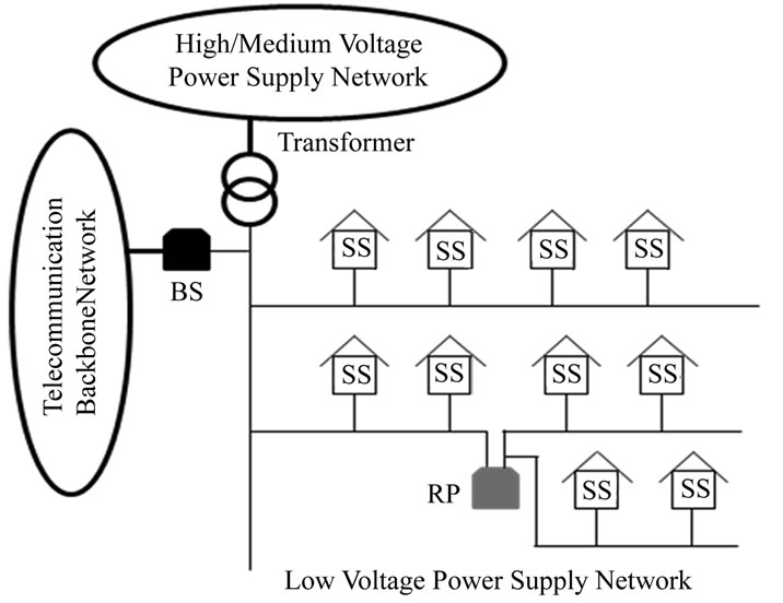
Figure 1. A PLC network model.
frequencies of interest for communications is usually very large in power lines. The RP is used for increasing signal strength when it falls below some predefined value.
The BS is an access point for the communications between an SS of the PLC network and a user of an external network, as well as the communications between the SSs inside the PLC network. The signal transmission directions in a PLC network include downlink—from the BS to the SSs and uplink—from an SS to the BS. In the downlink, the BS sends a transmission signal to all the SSs in the PLC network. In the uplink, a signal sent by an SS can not only be received by the BS, but also be received by all other SSs. Hence, the PLC access network holds a logical bus topology, where a set of SSs are connected via a shared communication media—power line, called bus. This type of network may have problems when two or more SSs want to transmit at the same time on the same bus. Hence, some scheme of collision handling or collision avoidance is required for communications, such as carrier sense multiple access (CSMA) or an access control by the BS. The latter is assumed here.
The OFDM is recommended by ITU-T G.hn as the modulation scheme for PLC networks due to the fact that it can cope with frequency selectivity (or time dispersion)—the most distinct property of power line channel, without complex equalization filters. Moreover, the OFDM can perform better than single carrier modulation in the presence of impulsive noise, because it spreads the effect of impulsive noise over multiple subcarriers. The available spectrum is divided into a set of narrowband subcarriers (or subchannels), say m, which are overlapping in frequency and orthogonal in time. We assume that these m channels are all traffic channels. The signaling control is assumed to be ideal and not discussed here.
As mentioned in [4,5], the impulsive noise introduces significant time variance into the power line channel, which indicates a high likelihood of bit or even burst errors for digital communications over power lines. The statistics of the measured interarrival times of impulsive noise above 200 ms follows an exponential distribution. Probably for this sake, the channel was modeled by a Markov chain with two states in [6], Ton and Toff, represented by two exponentially distributed random variables, where Ton denotes the absence of impulses and the channel is available for utilization, and Toff denotes the duration that the channel is disturbed by an impulse and no information transmission is possible. In this work, we shall follow the same assumption for the distribution of interarrival times of impulsive noise.
The BS knows about the occupancy status of the channels and allocates the available channels to the requested calls from the SSs. When a requested call arrives, it will occupy one channel for communication if there is one available; however, it will wait in a buffer if all the m channels are occupied. The waiting calls are served in first-come first-served (FCFS) order. The head-of-line (HOL) waiting call will get service as soon as an idle channel becomes available. Assume that there is no upper bound for the waiting time. Note that the considered PLC network has a finite population N with m traffic channels (In principle, N > m), the number of calls in the buffer usually does not exceed the value N – m, in general. We set the buffer size as N – m.
Note also that the channels are subject to failure during service due to the noise/disturbance. The failure events in different channels are independent and identically-distributed (i.i.d.). When a channel happens to be in failure, its associated call will be dropped from the system. We remark that for modeling purpose, the call can also be placed into the buffer. However, we select the former case to give the SS an extra choice. The SS can choose either to initiate or not to initiate a new call request. If the call is initiated as a new call request, it may get an immediate service when there is one channel available, or be placed into the buffer when all the m channels are not available. Once the failed channel is recovered, i.e., the disturbance is gone, the channel will become available for the HOL call in the buffer.
3. Performance Analysis
For the above PLC network with N SSs and m traffic channels, we assume that the arrival process of an individual idle SS is a Poisson process with rate λ. The channel holding time of a call is exponentially distributed with mean 1/μ. We further assume that each call occupies one channel for simplicity. However, the analysis method used here can be extended to handle bandwidth requests of variable size (cf. [17]).
Due to noise/disturbance, the channel may be subject to failure. The interarrival time of the failure events is assumed to follows exponential distribution with mean 1/α. In each failure event, it is assumed that the remaining duration (i.e., the recovery time) is exponentially distributed with mean 1/β.
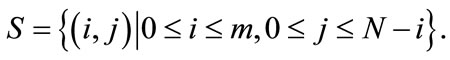
Let X(t) be the number of failed channels at time t. Similarly, let Y(t) be the number of calls in the system at time t, including the calls being served and those waiting in the buffer. The process (X(t), Y(t)) is a two dimensional Markov process with state diagram as shown in Figure 2 and state space
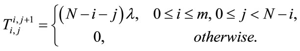
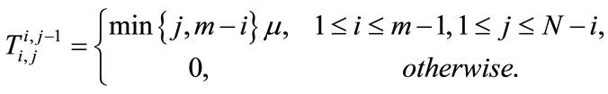
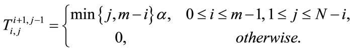
Different transition rates from state (i,j) to (i',j') are specified as follows.
 (1)
(1)
 (2)
(2)
 (3)
(3)
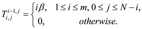 (4)
(4)
Let π(i,j) denote the steady-state probability that the PLC network is at state (i,j). The global balance equations of the system are given as follows:
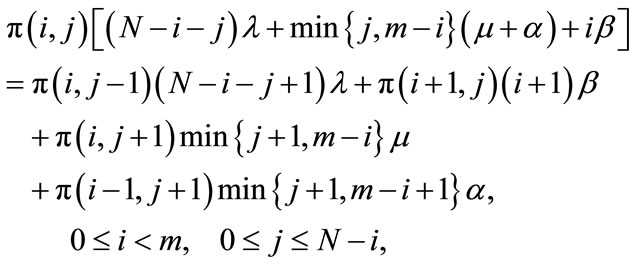 (5)
(5)
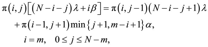 (6)
(6)
where ,
,  , and
, and  if
if . The above equations contain
 unknowns, i.e., the probabilities π(i,j) with
 , and
, and , of which, however, there are only
  independent equations. Thus, (N + 1) more equations are required to solve the problem.
Observing the structure of Figure 2, it is found that only the first row exists if α = 0 and β = 0. From [18, Chapter 5], we can determine a set of particular solutions, π(0,j), j = 1, 2, …, N, as follows.
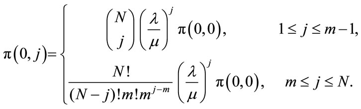 (7)
(7)
The final equation is provided by the normalization condition:
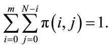 (8)
(8)
Equations (5)-(8) are sufficient to evaluate the state probabilities π(i, j).
4. Performance Metrics
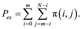
4.1. The Probability that All Channels are not Available
The probability that all channels are not available (either in service or in failure), denoted by Pex, is the sum of the state probabilities with i + j ≥ m. This event is seen by an external observer.
 (9)
(9)
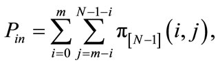
4.2. The Probability that an Initiating SS Must Wait for Service
This is the probability that the initiating SS finds all channels not available (either in service or in failure) when placing a call request, denoted by Pin. This metric is similar to Pex except that the observer is an internal source. Note that the proposed model is a finite source system, the PASTA property does not hold. By using the arrival theorem [19, Section 6.2.4], the Pin that one of the N SSs finds all channels not available when placing a call request is obtained by replacing N with N – 1 in (9).
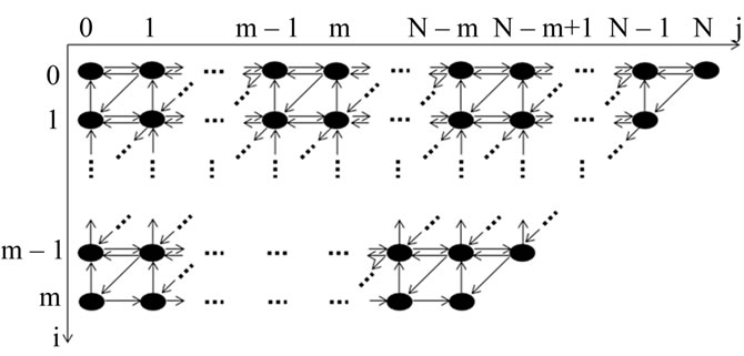
Figure 2. The state diagram of the PLC network (N > 2 m case).
 (10)
(10)
where  denotes the steady state probability at (i,j) when the total number of SSs in the network is N-1. Following this notation, the Equation (9) can be re-written as

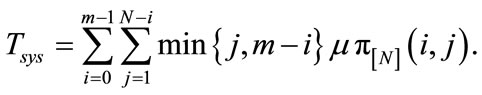
4.3. The Mean System Throughput
The mean system throughput, denoted by Tsys, is defined as the mean number of calls being served per unit time.
 (11)
(11)
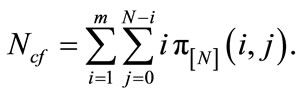
4.4. The Mean Number of Channels in Failure
The mean number of channels in failure, denoted by Ncf, is defined as the mean number of failed channels in steady state.
 (12)
(12)
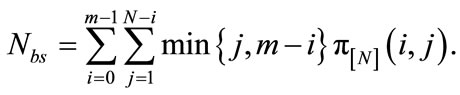
4.5. The Mean Number of Calls
Here we study the mean number of calls being served, denoted by Nbs, and the mean number of calls waiting at the buffer, denoted by Nwb. They are obtained as follows.
 (13)
(13)
 (14)
(14)
By adding them together, we obtain the mean number of calls in the system, denoted by Ntot.
 (15)
(15)
4.6. The Waiting Time Distribution
As mentioned earlier, a requested call from an SS will wait in the buffer when it finds no channel available. The waiting calls can get service in accordance with FCFS discipline when a channel becomes available. We now study, for each time t ≥ 0, the probability P(W > t) that a given SS waits in excess of t before receiving service, where the given SS is referred to as the test SS (or test call), and the random variable W is the test call’s waiting time.
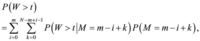
Without loss of generality, we assume that the test call finds all the m channels not available with i channels in failure (i.e., m – i calls in service), and k, 0 ≤ k ≤ N – (m – i) – 1, other calls waiting in the buffer, when it initiates a request for service. The complementary waiting time distribution can be expressed as
 (16)
(16)
where M is the number of calls present in the system just prior to the test call.  is the probability that the test call finds all the m channels not available, i channels in failure, and k other calls waiting in the buffer, when it initiates a request. Thus, we have
 (17)
(17)
The conditional probability  is the probability that the test call waits beyond t when initiating a request, given all the m channels not available, i channels in failure and k other calls waiting in the buffer. In the FCFS discipline, the waiting time of the test call that finds all the m channels not available, i channels in failure and k other waiting calls ahead of it is the sum of the times that each of the k + 1 calls spends at the head of the queue. In other words, the test call can receive service only if the k + 1 calls ahead of it complete their service.1
We start the analysis from the system state  that the test call finds all the m channels not available, i channels in failure and k other calls waiting in the buffer. Let Z(t) be the number of calls waiting in the buffer at time t, the two processes (X(t), Z(t)) and (X(t), Y(t)) are equivalent at the condition that all the m channels not available, where X(t) and Y(t) have been defined in Section 3. For the new process (X(t), Z(t)), we can use (i, k) to represent the case that the test call finds all the m channels not available, i channels in failure and k other calls waiting in the buffer. Due to possible channel failure, the state (i, k) may generate some associated states with “k other calls waiting in the buffer”: (i + 1, k), (i + 2, k), ···, (m,k), as shown in Figure 3. We refer to the column of the state (i, k) and its generated states as Mode k, to emphasize the k waiting calls in the buffer. In each state of Mode k, either of the following two events can change Mode k to Mode (k-1) (i.e., all the m channels not available, i channels in failure and k – 1 other waiting calls in the buffer):
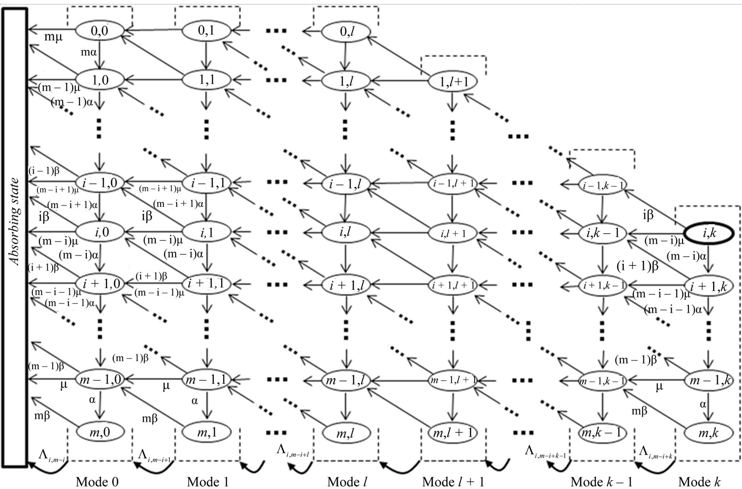
Figure 3. The phase process starting from mode k.
• When a call completes its service, it leaves the system and the HOL call in the buffer immediately receives service, and thus the number of calls in the buffer is reduced by 1.
• When a failed channel is recovered, the available channel is immediately occupied by the HOL call in the buffer and the number of calls in the buffer is reduced by 1.
Similarly, in each state of Mode (k – 1), either of the above two events changes the mode to Mode (k – 2). This procedure continues until the k + 1 calls ahead of the test call complete their service.
Since the service time and recovery time are assumed to be exponentially distributed and are independent of each other, the rate from each state of one mode, e.g., Mode l, to a corresponding state of the next mode, e.g., Mode (l – 1), is Poisson rate of a multiple of μ or a multiple of β, respectively [19, Theorem 2.3-2]. Hence, the total transition rate from Mode l to Mode (l – 1), denoted by ,2 can be determined, in steady state, by the superposition of all the Poisson rates weighted by respective state probabilities. After some mathematics, we obtain
 , 0 ≤ l ≤ k, as
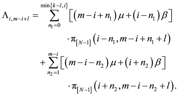 (18)
(18)
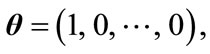
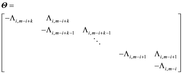
Since the time intervals between different adjacent modes are independent, the waiting time W of the test call at the condition that it finds all the m channels not available, i channels in failure and k other calls waiting in the buffer is phase-type distributed with k + 1 phases to enter the absorbing state (See Figure 3). The distribution of the waiting time W from the start of the phase process (i.e., Mode k, which is sourced from the system state (i, m – i + k)) until the absorbing state can be represented by  [20], where θ is a row vector of dimension k + 1, and
  is a square matrix of dimension k + 1, given by
Therefore, the conditional probability  and its mean can be expressed as
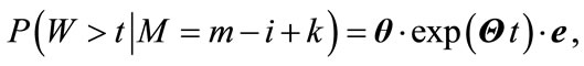 (19)
(19)
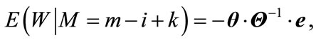 (20)
(20)
where e is a column vector of all ones. Substituting (17) and (19) into (16), we obtain the complementary waiting time distribution as
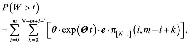 (21)
(21)
and the mean waiting time as
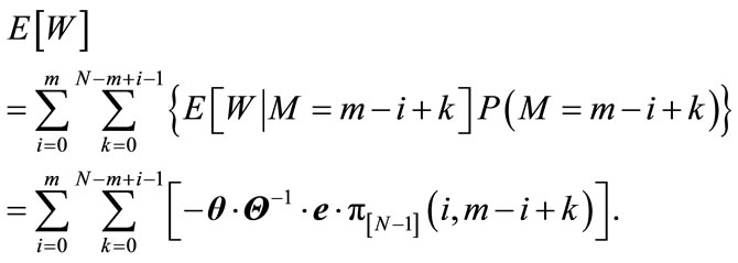 (22)
(22)
It is worthy to note that in Figure 3, for each state of Mode l, 0 ≤ l ≤ k – 1, although there is an arrival of call request (not shown in Figure 3) that makes the state transition to a corresponding state of mode (l + 1), this request is queued behind the test call, which does not affect the phase process to the absorbing state.
5. Numerical Results
In this section, we present the numerical results for the obtained performance metrics under the following configuration: N = 40, m = 10. The arrival rate of an individual idle SS λ changes from 1 to 8. The other parameters μ, α, and β are set separately with variable values in each figure. Note that all parameters are given in dimensionless units, which can be mapped to specific units of measurement.
To validate our analysis, we also developed a discrete event simulator for the proposed model. The simulation was implemented in MATLAB. For convenient illustration, we only show one group of simulation results as a comparison. In the illustrated figures, an excellent match between the analysis and simulation can be observed. Each simulated data point was averaged over 5,000 trials and the 95% confidence intervals were computed.
Figure 4 shows how the probability Pex changes with various parameters. We observe that Pex increases with the increase of call arrival rate λ, or the service time 1/μ.
As λ increases, the system is easier to get full channel occupancy. As the service time increases, the system becomes more difficult to release a channel. In our parameter configuration, we also observe that Pex decreases when α is increased. At the first sight, the increase of α would delay the channel availability. However, in the model, the call in service will be dropped when a channel fails; once the channel is recovered, the channel will become available and benefit the initiating calls. Thus, there is a tradeoff impact of α, depending on dominance between the recovery time and the residual service time. In our configuration, the recovery time is much faster than the residual service time, which leads to the decrease of Pex. Similarly, for the impact of β on Pex, there is also a tradeoff. We observe that the decrease of β may cause Pex to decrease in some case (e.g., β is set from 100 to 80), and cause Pex to increase in some other case (e.g., β is set from 80 to 30).
Figure 5 shows how the probability Pin changes with various parameters. The performance curves are similar to that in Figure 4 due to the same reason.
Figure 6 shows how the mean system throughput Tsys changes with various parameters. We observe that Tsys increases with the increase of λ or the service rate μ, and decreases with the increase of channel failure rate α or the required recovery time 1/β. As the call arrival rate or the call service rate increases, the mean number of calls processed per unit time will be increased. A more frequent channel failure event or a longer required recovery time will negatively affect the performance of the system throughput.
In Figure 7, we observe that the mean number of channels in failure, Ncf, increases with the increase of λ and decreases with the increase of μ. As λ increases, more calls occupy the channels per unit time, leading to more channels subject to failure. Note that in our model, it is assumed that the channels are subject to failure during service. We do not consider the failure events for idle channels due to no calls in service (although there are a little impact to an initiating call that happens to access an idle channel being in failure). As μ increases, a call completes its service in shorter duration, reducing the chance for a call to encounter a channel failure event. We also observe that Ncf increases with the increase of channel failure rate α or the required recovery time 1/β. The reason is obvious.
In Figure 8, we observe that the mean number of calls
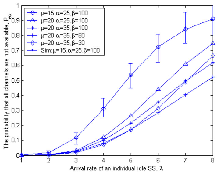
Figure 4. The probability that all channels are not available to the initiating calls, Pex.
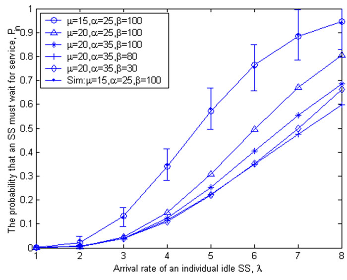
Figure 5. The probability an initiating SS must wait for service, Pin.
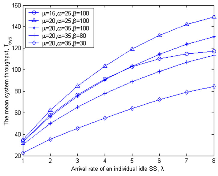
Figure 6. The mean system throughput, Tsys.
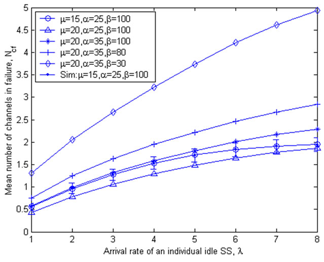
Figure 7. The mean number of channels in failure, Ncf.
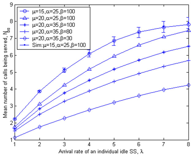
Figure 8. The mean number of calls being served, Nbs.
being served, Nbs, increases with the increase of λ, and decreases with the increase of μ. This agrees with our intuition. As λ increases, a snapshot in steady state will capture more calls being served. On the other hand, the larger the $\mu$, the faster the processing time of a call in service, and thus less calls in service can be captured by a snapshot. We also observe that Nbs decreases with the increase of channel failure rate α or the required recovery time 1/β. As α is increased or β is decreased, a snapshot in steady state will capture less calls being served.
In Figure 9, we observe that the mean number of calls waiting at the buffer, Nwb, increases with the increase of call arrival rate λ or service time 1/μ. As λ increases, the system becomes full more quickly, leading to more subsequent calls entering the buffer. As μ decreases, a call needs longer time to complete its service, giving less chance for the waiting calls to move out of the buffer. Similar to Figure 4, there are also tradeoffs for the impact of α and β on Nwb. In our configuration, we observe that Nwb increases with the increase of α or β at a relatively large value of β. When β is too small, i.e., the required recovery time is too large, this parameter dominates in all factors and tends to increase the number of waiting calls in the buffer, as compared by the two cases of (μ = 20, α = 35, β = 30) and (μ = 20, α = 35, β = 80). For the impact of α, on one hand, a channel failure event inherently delays the time for a waiting call to capture an idle channel; on the other hand, when α increases, the number of dropped calls from the failed channels is increased, leading to more chance for the waiting calls, once the channels are recovered, to move out of the buffer.
Figure 10 shows the complementary waiting time distributions with respect to time t, obtained under different parameter configurations. We observe that the waiting time increases when λ increases and decreases when μ increases. Similar to Figure 9, there are also tradeoffs for α and β. In our configuration, we observe that the waiting time of the test call decreases with the increase of either α or the required recovery time 1/β. The reason can be
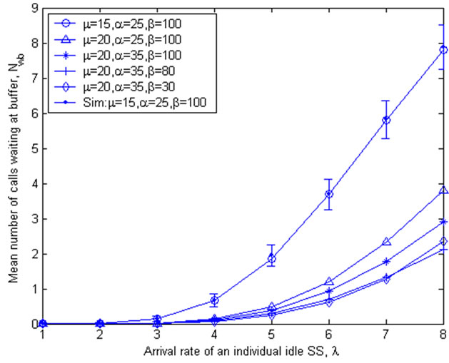
Figure 9. The mean number of calls waiting at buffer, Nwb.

Figure 10. The complementary waiting time distributions, P(W > t).
referred to Figure 9. In addition, we may directly see the impact of β from Fig. 9 by the two cases of (μ = 20, α = 35, β = 100) and (μ = 20, α = 35, β = 80): as the required recovery time increases, the mean number of waiting calls at the buffer, Nwb, decreases; thus, the waiting time of the test call naturally decreases.
6. Conclusions
We analytically modeled a general finite-source PLC network subject to channel failure and evaluate its performance at the call-level through a queueing theoretic framework. The proposed PLC network model consists of a BS, which is located at a transformer station and connected to the backbone communication networks, and a number of SSs that are interconnected with each other and with the BS via the power lines. An OFDM based transmission technique is assumed to be used for providing the transmission channels in a frequency spectrum, which is divided into a set of narrowband subchannels. The channels are subject to failure during service due to noise/disturbance.
We determined the steady-state solution of the proposed model and derived a set of performance metrics of interest, such as the probability that all channels are not available (either in service or in failure), the probability that an initiating SS must wait for service, the mean system throughput, the mean number of channels in failure, the mean number of calls being served, the mean number of calls waiting at the buffer, and the waiting time distribution of the queued calls. Numerical results and detailed discussion were presented to show the impact of system parameters on the derived performance metrics.
The proposed modeling method and the derived metrics are expected to be used for evaluation and design of future PLC networks.
REFERENCES
- ITU-T Recommendation G. 9960, Unified High-Speed Wire-Line Based Home Networking Transceivers—Foundation, 9 October 2009.
- IEEE P1901 Draft Standard, Broadband over Power Line Networks: Medium Access Control and Physical Layer Specifications, January 2010.
- M. Stantcheva, K. Begain, H. Hrasnica and R. Lehnert, “Suitable mac protocols for an OFDM based PLC network,” 4th International Symposium on Power-Line Communications and its Applications (ISPLC 2000), Limerick, 5-7 April 2000.
- M. Zimmerman and K. Dostert, “The Low Voltage Power Distribution Network as Last Mile Access Network— Signal Propagation and Noise Scenario in the HF-Range,” International Journal of Electronics and Communications (AEU), Vol. 54, No. 1, 2000, pp. 13-22.
- M. Zimmerman and K. Dostert, “Analysis and Modeling of Impulsive Noise in Broad-Band Powerline Communications,” IEEE Transactions on Electromagnetic Compatibility, Vol. 44, No. 1, February 2002, pp. 249-258. doi:org/10.1109/15.990732
- H. Hrasnica and A. Haidine, “Modeling MAC Layer for Powerline Communications Networks,” 4th International Symposium on Power-Line Communications and its Applications (ISPLC 2000), Limerick, 5-7 April 2000.
- K.-R. Lee, J.-M. Lee, W.-H. Kwon, B.-S. Ko and Y.-M. Kim, “Performance evaluation of CSMA/CA MAC Protocol in Low-Speed Plc Environments,” 7th International Symposium on Power-Line Communications and its Applications (ISPLC 2003), Kyoto, 26-28 March 2003.
- M. Chung, M.-H. Jung, T.-J. Lee and Y. Lee, “Performance analysis of homeplug 1.0 mac with CSMA/CA,” IEEE Journal on Selected Areas in Communications, Vol. 24, July 2006, pp. 1318-1325.
- D. Umehara, S. Hirata, S. Denno and Y. Morihiro, “Modeling of Impulse Noise for Indoor Broadband Power Line Communications,” International Symposium of Information Theory and Its Applications (ISITA 2006), Seoul, October 2006.
- M. Katayama, T. Yamazato and H. Okada, “A Mathematical Model of Noise in Narrowband Power Line Communication Systems,” IEEE Journal on Selected Areas in Communications, Vol. 24, No. 7, 2006, pp. 1267-1276. doi:org/10.1109/JSAC.2006.874408
- J. Haring and H. Vinck, “OFDM Transmission Corrupted by Impulsive Noise,” 4th International Symposium on Power-Line Communications and Its Applications (ISPLC 2000), Limerick, 5-7 April 2000.
- C. L. Giovaneli, B. Honary, P. Farrell and P. Benachour, “Collaborative Coding Multiple Access Communications for Power Line Channels,” 7th International Symposium on Power-Line Communications and its Applications (ISPLC2003), Kyoto, 26-28 March 2003.
- P. Amirshahi, S. Navidpour and M. Kavehrad, “Performance Analysis of Ofdm Broadband Communications System over Low Voltage Powerline with Impulsive Noise,” Proceeding of IEEE ICC’06, June 2006, pp. 367-372.
- M. Ferreiro, M. Cacheda and C. Mosquera, “A Low Complexity All-Digital DS-SS Transceiver for Power-Line Communications,” 7th International Symposium on PowerLine Communications and Its Applications (ISPLC 2003), Kyoto, 26-28 March 2003.
- J. Yu, H. Yu and Y.-H. Lee, “Design of a Power-Line Modem for Monitoring and Control Systems,” 7th International Symposium on Power-Line Communications and its Applications (ISPLC 2003), Kyoto, 26-28 March 2003.
- K. Begain, G. Bolch and H. Herold, Practical Performance Modeling—Application of MOSEL Language, Kluwer Academic Publishers, Dordrecht, 2000.
- S. Tang and W. Li, “An Adaptive Bandwidth Allocation Scheme with Preemptive Priority for Integrated Voice /Data Mobile Networks,” IEEE Transactions on Wireless Communications, vol. 5, No. 10, October 2006, pp. 2874- 2886. doi:org/10.1109/TWC.2006.04632.
- P. G. Harrison and N. M. Patel, Performance Modelling of Communication Networks and Computer Architectures, Addison-Wesley, Boston, January 1993.
- H. Kobayashi and B. L. Mark, System Modeling and Analysis: Foundations of System Performance Evaluation. Pearson Education, Inc., Upper Saddle River, 2009.
- L. Breuer and D. Baum, An Introduction to Queueing Theory and Matrix-Analytic Methods, Springer, Dordrecht, December 2005.
NOTES
1We ignore the case when the k + 1 calls ahead of the test call complete their service, the available channel for the test call suddenly fails. In that case, the waiting time should be added by an extra time, which is the minimum of the channel recovery time and the residual time of the next completed call.
2The subscript represents that the test call finds all the m channels not available, i channels in failure and l other calls waiting in the buffer.