World Journal of Mechanics
Vol.1 No.3(2011), Article ID:5777,10 pages DOI:10.4236/wjm.2011.13018
The Electrokinetic Cross-Coupling Coefficient: Two-Scale Homogenization Approach
1Lavrentyev Institute of Hydrodynamics, Novosibirsk, Russia
2Trofimuk Institute of Petroleum-Gas Geology and Geophysics, Novosibirsk, Russia
E-mail: Shelukhin@list.ru
Received April 7, 2011; revised May 9, 2011; accepted May 19, 2011
Keywords: Electroosmosis, Two-Scale Homogenization, Cross-Coupling Coefficient
ABSTRACT
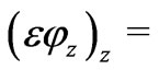
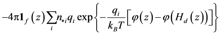
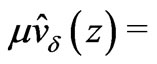
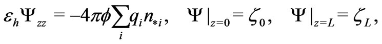
By the two-scale homogenization approach we justify a two-scale model of ion transport through a layered membrane, with flows being driven by a pressure gradient and an external electrical field. By up-scaling, the electroosmotic flow equations in horizontal thin slits separated by thin solid layers are approximated by a homogenized system of macroscale equations in the form of the Poisson equation for induced vertical electrical field and Onsager's reciprocity relations between global fluxes (hydrodynamic and electric) and forces (horizontal pressure gradient and external electrical field). In addition, the two-scale approach provides macroscopic mobility coefficients in the Onsager relations. On this way, the cross-coupling kinetic coefficient is obtained in a form which does involves the  -potential among the data provided the surface current is negligible.
1. Introduction
In numerous studies on the electrolyte flows in rocks, the pore pressure  and the streaming (electric) potential
  interplay through the equation
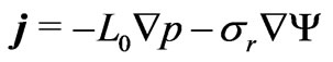 , where
  is the current density,
  is the saturated rock conductivity, and
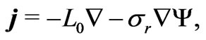
  is the electrokinetic cross-coupling term. Hydrogeological applications concern the study of water leakage from dams [1], groundwater flows in geothermal fields and volcanoes [2], estimation of water resources [3]. In electrochemistry, the above equation form a basis for managing microchip separations of analytes in nano-channels [4]; there is also an evidence that this equation find applications in hydrocarbon recovery [5,6].
By the Helmholtz-Smoluchowski theory [7], the term  is given by the formula
 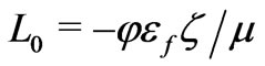 where
where  is the porosity,
  is the dielectric permittivity of the saturating fluid,
  is the viscosity, and
  is the so-called
  -potential, the electric potential across the diffuse part of the interfacial double layer. In [8,9,10], the above formula is substituted by
 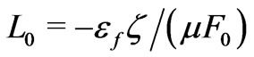 (or more sophisticated formulas), with
 being a dimensionless formation factor.
The goal of the present paper is to give more mathematical insight into the physico-chemical nature of the cross coupling coefficient . Restricting ourselves to one-dimensional flows, we derive a representation formula for
 by the two-scale homogenization technique [11,12], starting from the equations of the ions transport through a layered membrane with a periodical structure. On this way we arrive at electro-osmotic macro-equations, whereas electrokinetic coupling coefficients can be determined from micro-equations defined on the periodicity cell.
Homogenization is a process in which the composite material with microscopic structure is replaced by an equivalent material with macroscopic, homogeneous properties. There are two methods of up-scaling coupled equations at the microscale to equations valid at macroscale for fluid-saturated porous media. The first is the volume averaging and the second is the two-scale and multiscale homogenization. Volume averaging has been applied successfully to derive the form of Biot's equations of poroelasticity [13], and a wide variety of other up-scaling problems in double-porosity poroelasticity [14]. The averaging theorem used by all these authors is due to J. C. Slattery (1967) [15] and is based on well-known Green's theorem together with the idea that in relatively small regions volume averages of spatial gradient in statistically homogeneous media are presumably closely related to gradient of volume averages.
The two-scale homogenization method requires that the heterogeneous microstructure of a rock sample is described by spatially periodic parameters and the microscale of the heterogeneous porous medium is much smaller than the macroscale of most interest. The approach involves assuming that any quantity can be treated as a function of a macroscale variable and a microscale variable. The two-scale homogenization is a well established method in the theory of partial differential equations with rapidly oscillating periodic coefficients. This method has a lot of important applications in various branches of physics, mechanics and modern technology: porous media, composite and perforated materials, thermal conduction, acoustics, electromagnetism. For general references on the homogenization theory we refer to [12,16,17,18].
The two-scale homogenization method can give formulas for coefficients in the up-scaled equations, whereas volume averaging methods give the form of the up-scaled equations but generally must be supplemented with physical arguments and/or data in order to determine the coefficients. A more detailed comparison of two up-scaling methods can be found in [19].
The present study is applicable to sandstones if surface conductivity can be neglected. When passing to claycontaining rocks one should also take into account bound charges concentrating on the interface surfaces. Such rocks are not considered here.
2. Background
Within the frame of the nonequilibrium thermodynamics, the fluxes (the Darcy's volume fluid velocity  and the electric current density
 ) are derived as a linear combination of thermodynamical forces (the pressure gradient
  and the electric potential gradient
 ):
):
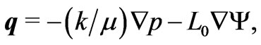 (1)
(1)
 (2)
(2)
where  is the permeability. Our goal is to show that these equations, specified for one-dimensional flows through a layered membrane, can be derived by the two-scale homogenization technique starting from the equations valid at microscale. While deriving the up-scaled equations (1) and (2), (which can trace back to Helmholtz and von Smoluchowski) we obtain a formula for the cross-coupling coefficient
 .
.
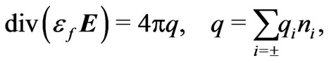
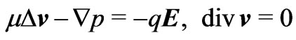
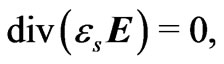
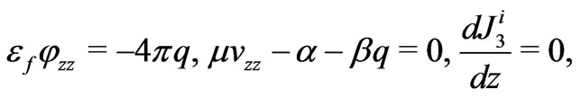
In this section, we summarize equations that govern the flows of a binary electrolyte solution through the pore space of a solid dielectric. To make clear our hypotheses on physical parameters, we use the Gaussian system of units. Clearly, while comparing final calculations with experiments, we apply the SI units. The electric field E obeys the charge conservation law
 (3)
(3)
where  is the fluid dielectric permittivity,
 is the charge of a positive ion,
 is the charge of the negative ion,
  is the ion concentration. Viscous incompressible flows of the electrolyte solution is governed by the Navier-Stokes equations [7]
 (4)
(4)
with the inertial terms being neglected in the first momentum equation. Here,  is the velocity of the bulk fluid. The motion of both the ionic species satisfies the transport equation

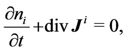 (5)
(5)
with the flux given by the Nernst-Plank relation [7]
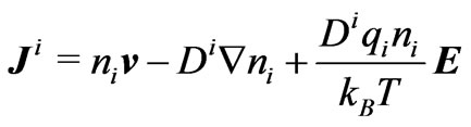
where  is the diffusion coefficient,
  is the Boltzmann constant,
  is the absolute temperature.
Inside the solid dielectric, the electrical field obeys the equation
where  is the solid dielectric permittivity. In what follows,
  stands for the electric potential,
 .
.
The solid-fluid boundary conditions will be formulated below for one-dimensional flows.
3. One-Dimensional Flows
To motivate our further study we keep in mind a vertical membrane of thickness  (see Figure 1) when the inflow pressure
  (on the left) is grater than the outflow pressure
 . It is the pressure gradient
  which mainly controls the flow. It is also possible that the flow is due to the external electrical field
 . Commonly, an inflow concentration
  of the
  -th ion is prescribed on the left.
Now, to perform analytical study of the flow equations, we consider a vertical "membrane" of an infinite thickness. We study electrolyte steady flows through the horizontal layer of thickness  consisting of
  horizontal thin slits
  of the same thickness
  separated by layers
  of a solid
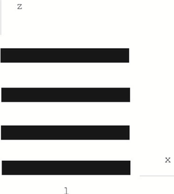
Figure 1. Layered membrane of the thicknes  consisting of
  solid/liquid layers.
dielectric of the same thickness . The central points
  of the liquid intervals
  are the points of reference where the ion inflow densities
  take the prescribed values
 .
.
Let  and
and  stand for fluid and solid domains
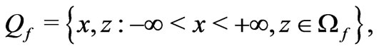
In the domain , we look for steady solutions of the fluid Equations (3-5) in the form
where  and
and  are given constants. Under these assumptions, Equations (3-5) in each fluid interval
  become
 (6)
(6)

We study horizontal flows along the  -axis, hence
 . The latter equality is equivalent to
Integrating between  and
and , we exclude the concentration functions from consideration by the formula
In the solid intervals , the potential
  satisfies the equatio
 (7)
(7)
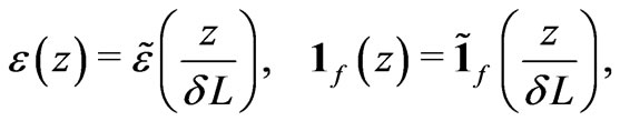
In what follows we assume that the dielectric permittivity function and the fluid indicator function
are extended periodically on the real line . Given a function
  continuous everywhere except a point
 , we introduce the jump as follows
In some sandstones, surface conductivity can be neglected depending on the pore water salinity and the cation exchange capacity of the mineral surface. For such sandstones, the “electric” boundary conditions reduce to the conditions of continuity of the potential  and the normal component the electric induction vector
 :
:
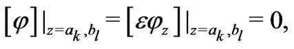 (8)
(8)
where k = 1,…, n-1 and l = 0,…, n-1.
The velocity satisfies the no-slip conditions
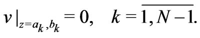 (9)
(9)
We assume that  satisfies the external boundary conditions
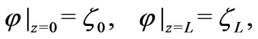 (10)
(10)
with the prescribed  -potentials
  and
and . We introduce a function
 , which takes the value of the integer part of the number
 . Then the functions
take constant values  for
for . Thus to define
  on the whole interval
 , one should solve the non-local Poisson-Boltzmann equation
 (11)
(11)
jointly with the conditions (8) and (10). Observe that the function  is periodic, and
  on the interval of periodicity
 .
.
With the function  at hand, one can find a velocity
  from Equations (6) and the boundary conditions (9).
4. Nondimensionalisation
We look for an asymptotic solution of problem (11), (8), (10), (6), (9) for the functions  and
and , assuming that the ratio
  is a small parameter for some positive entire number
 . We argue by the homogenization approach [24], so the entire interval
  is fixed and
  varies in
 . In that case
  and
and

Here,  is the porosity.
We call  a slow variable and we introduce the fast variable
 . With
  being small, the periodic functions
  and
and  oscillate strongly and they can be represented as functions of the fast variable:
where
are periodic functions with the period equal to 1. In what follows the functions
and
are extended periodically for all . The functions
 ,
,  ,
,  can be written as
and
In the notations used, the function  on the interval
  is a solution of the problem
 (12)
(12)

where 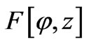 is equal to
It follows from Equations (6) that the bulk velocity satisfies the equation
 (13)
(13)
Let us perform scaling, using the symbol  for a reference value of the dimensional quantity
  and the symbol
  for a dimensionless quantity of
 , i. e.
 . We use the following notations:

The quantity
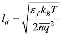 (14)
(14)
is known as the Debye length. In terms of dimensionless variables Equations (13) and (11) in the fluid domain  take the form
Here,
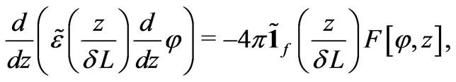
In the solid domain Equation (7) becomes 
Assuming that the dimensionless quantities  satisfy the equalities
we obtain a hierarchy of problems to study. In this paper we restrict ourselves to the case when all the powers  are equal to zero, i. e.
 . The meaning of these hypotheses is the following. The relation
  implies that electroosmotic force and thermal force are of the same order. Observe that the relation
  holds, for example, for the symmetric electrolyte (where
  and
and ) in water at
 , with the valency
  and with the
  -potential equal to
  [4]. When
  is not small, the Debye-Hückel linearization of the Poisson-Boltzmann equation does not work. Under the condition
  the Debye length
  can be longer compared to electrical double layer, moreover the double layer overlapping could occur. Indeed, it is a useful rule of thumb that
 [4] where
  is the valency. For the above mentioned electrolyte with the counterion molar concentration
  we have
 , whereas the double electric layer is normally only a few nanometers thick [4] and the nanocapillary membrane may have the pore diameter of 15
  [20]. For such cases the hypothesis
  is natural. Hypothesis
  amounts to the effect that the horizontal pressure gradient and the applied horizontal electrical field are of the same order. The relation
  means that viscous response is of the same order as the applied horizontal pressure gradient.
There is one more assumption that we impose on the Péclet number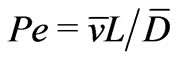 :
:
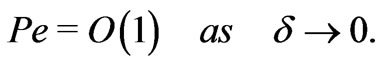 (15)
(15)
The hypothesis implies that convection and diffusion are of the same order.
We close this section by reminding the Debye-Hückel approach to the Poisson-Boltzmann Equation (11) in the single layer  with the boundary conditions
 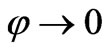 and
and  as
as  and
and . In the case of symmetric electrolyte, the linearized equation (11), in the SI system of units where
  is substituted by 1, becomes
 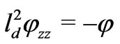 , since the nonlocal term
  vanishes as
 . Clearly,
  is a solution. This explains the notion (14).
5. Asymptotic Analysis of Electric Field
We proceed by returning to the dimensional variables. Using the method of the two-scale expansions [12], we look for the solution of Equation (12) in the form of an expansion series
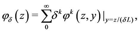 (16)
(16)
where the functions  are periodic in the variable
 ,
,  , with a period equal to 1 for each
 . We introduce the flux
 (17)
(17)
Clearly,
 (18)
(18)
We present this flux as a series
 (19)
(19)
where the functions  are 1-periodic in
  for all
 .
.
Using the formula
and substituting the series (16) and (19) into equality (17), we obtain an equality which looks like
Thus  for all
 . In particular, the three first equalities can be written as
and
Substituting the series (16) and (19) into equality (18) and paying attention to the powers  and
and , we obtain the equations
 (20)
(20)
 (21)
(21)
Equations (20) and (21) allow one to determine the functions ,
,  and
and  uniquely. Indeed, with a function
  independent of the variable
 , we look for
  by the method of separation of variables assuming that there exists a
  -periodic function
  such that
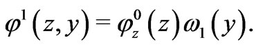
Substituting this presentation into equation (20), we find that the function  solves the following problem on the interval
 :
:
 (22)
(22)
The latter integral condition serves for uniqueness. We integrate and arrive at the formulas
 (23)
(23)
Next, we use periodicity and integrate equation (21) with respect to  to obtain the following macro-equation for
 :
:
 (24)
(24)
As for the function , we look it in the form
Substituting this presentation into equation (21), we find that  is a periodic solution of the problem
 (25)
(25)
This problem has a unique solution provided
Thus, we have established the following asymptotic equality for the electric potential:
 (26)
(26)
6. Asymptotic Analysis of Velocity
Integrating Equation (13), we obtain the following formula for velocity in each fluid domain :
:
where
We extent the function  by zero to the solid intervals and denote such an extension by
 . Now, with
  standing for
 , we have for all
  that
that
 (27)
(27)
With  given by the expansion series (16), we look for
  in the form
 (28)
(28)
where the functions  are
are  -periodic in
  and
and  for
for . After simple calculations, we find that
Using the properties of functions ,
,  ,
,  , we obtain that
  is equal to

for 
As for , we find that it is equal to
for 
By virtue of the multiplier  in the right side of equation (11), we can assume that
Then, the variables  belong to the interval
also. As  is between
  and
and , the inequalities
hold and the second derivatives of  in Equation (25) are meaningful. In addition, it follows from Equations (23), (24) and (25) that, for
 , the functions
  satisfy the equations
Thus, we obtain
 (29)
(29)
Substituting equations (28) and (29) into equation (27) and considering only the power , one can show that the function
  does not depend on the variable
  and has the form
 (30)
(30)
Integrating equation (30) over the periodicity cell, we obtain the macroscopic equation
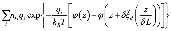
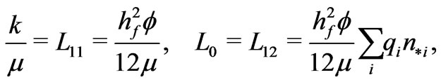
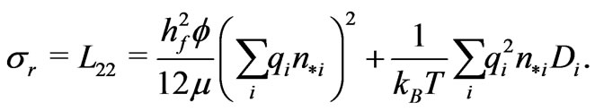
where the hydrodynamic and electrochemical mobilities are defined by the formulas
Thus, we have established the following asymptotic equality for the velocity field:
 (31)
(31)
We introduce the total electric current  whose horizontal component in the fluid phase is equal to
We extent the function  by zero to the solid intervals and denote such an extension by
 . Due to hypothesis (15), we have that
  . This is why we look for
  in the form of the expansion series
 (32)
(32)
It follows from (32) and (28) that

By integration, we arrive at the macroscopic equation
where  and
and

Thus, we have established the following asymptotic equality for the electric current:
 (33)
(33)
The asymptotic equalities (26), (31) and (33) are valid in the sense of weak or two-scale convergences; mathematical aspects of these asymptotic expansions are extensively investigated in [21,22,23].
7. Electrokinetic Coupling Coefficients
We introduce the Darcy volumetric flow rate  and the current density
 . By the above asymptotic analysis we have derived the macroequations (which are valid up to terms
 ,
, )
)
 (34)
(34)
which describe electrolyte flow and distribution of the electric potential  across a layered membrane under the assumption that
are prescribed data. For such a membrane, the effective dielectric permittivity  and the electrokinetic coupling coefficients
  are given by the formulas
 (35)
(35)
 (36)
(36)
 (37)
(37)
Formula (35) stating that the effective permittivity  of the layered membrane is the harmonic mean of
  and
and  was first derived by Maxwell (Maxwell 1881) in a different way [24]. Observe, that the Onsager reciprocity relation
  [25] is not imposed but derived in the above calculations as a consequence of the homogenization procedure. Moreover, the inequality
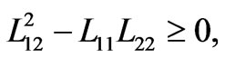 (38)
(38)
providing nonnegativity of the entropy production rate is also satisfied automatically [26] due to the representation formulas (36) and (37). The inequality (38) becomes equality if both the diffusion coefficients  are negligible. Observe that for some free solutions
  [27].
[27].
We emphasize that the coupling coefficients  in the macro-equations (34) are given by the representation formulas (36) and (37) as a result of an extensive analysis of the micro-equations (22) and (25) for the functions
  and
and  defined on the periodicity cell.
Clearly, the electroosmosis Equations (1) and (2) should coincide with the system (34) for onedimensional flows. Whereas the formula
for the cross-coupling coefficient have a drawback of measuring the  -potential, the kinetic coefficients
  derived by homogenization for the ideal (layered) porous medium do not depend on
 . One can exploit this advantage in calculation of the coupling coefficient
  for general porous media.
Applying the general Equations (1) and (2) to the ideal (layered) porous medium, we find that
Now, we have
 (39)
(39)
and inequality (38) gives the following estimate for the electrokinetic cross-coupling coefficient :
:
 (40)
(40)
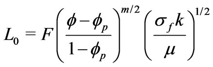
As for real rocks, formulas (39) and (40) suggest to take  in the form
 (41)
(41)
where  is a dimensionless geometrical factor. In applications, the above formula can be of use if no data are available for the diffusion coefficients
  and the
  potential. We emphasize that formula (41) is not a physical law but rather an engineering formula which can be of help for some sandstones when surface conductivity can be neglected.
Firstly, we evaluate  for a rock sample on the basis of the F.F. Reuss experiment [28]. Such an experiment reveals that a difference in the electric potentials
  applied to water in a U-tube results in a change of water levels when the low part of tube is plugged with a sandstone sample (Figure 2).
We calculate the weight  of salt water which fills the cylinder of height
  with cross section area
  (Figure 2). We have
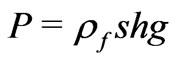 , where
  is the
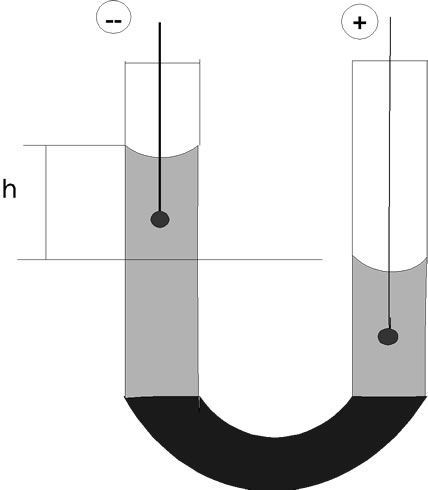
Figure 2. F. F. Reus experiment (1808) with the U-tube plugged with sandstone sample: applied electric field results in water level change of height
gravitational acceleration and  is the water density. The pressure drop across the sandstone plug is equal to
 . On the other hand it follows from Equations (34) that at equilibrium, when
 , we have
 .
.
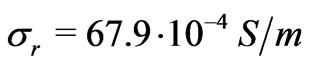
In [29,30], a mathematical model (jointly with a computer code) is developed for calculation of the electric conductivity  of a saturated rock. The model allows one to find an optimal Archie-like law
where  is the conductivity of the saturating fluid,
  is the percolation threshold porosity,
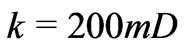
  is the cementation factor. For sandstones, it was calculated in [29] that
  0.03,
0.03,  1.5. Thus, for sandstones, formula (41) becomes
Now, the factor  can be evaluated from the formula
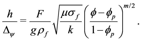
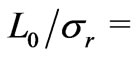
We perform calculation assuming that, as in [31], the applied potential difference 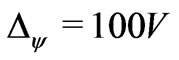 results in the water level difference
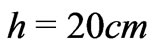 . The rock data are taken from [6]:
 ,
, ,
,  ,
,  ,
, . With these data at hand, we find that
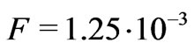 . It is the cross-coupling coefficient
 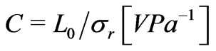 that can be measured in applications [32]. With the factor
  given above, we find that
 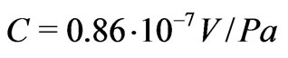 in agreement with the data in [6].
Next, we calculate the factor  for the rock sample composed of Berea sandstone 500 starting from experimental measurements of streaming potential when a fluid, with a prescribed NaCl concentration (500 ppm), flows through the sample [5]. Given data
 ,
,  ,
, ,
,
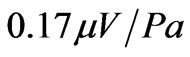 , we find from formula (41) that
 .
.
8. Conclusions
We have proposed a two-scale model for one-dimensional horizontal electroosmotic flows in a number of thin horizontal slits, with a horizontal pressure gradient and a horizontal electrical field being driving forces. The model is derived within the framework of homogenization in the up-scaling of the pore-scale description consisting of Stokes equation for bulk fluid flow and the Nernst-Plunk equation for the ion transport. The homogenized model is a generalization both of the Darcy law and the Ohm low. According to this model, both the fluid flux and the electric flux depend linearly on the horizontal pressure gradient and the horizontal electrical field, with the coupling coefficients obeying the Onsager symmetry condition and not depending on the  - potential.
As for three-dimensional general flows in sandstones in the case when surface current is negligible, the cross-coupling coefficient  is obtained in the approximate form
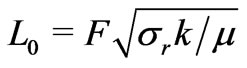 , where
  is the fluid saturated rock electric conductivity,
  is the rock permeability,
  is the fluid viscosity, and
  is dimensionless geometrical factor which depends on the sample. We evaluated that
 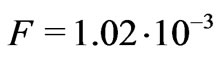 for Berea sandstones.
9. Acknowledgements
The authors were supported by Russian Fund of Fundamental Researches (grant 10-05-00835-a) and State Contract No. 14.740.11.0355 of Federal Special-Purpose Program “Personal”.
REFERENCES
- A. Bolève, A. Crespy, A. Revil, F. Janod and J. I. Mattiuzzo, “Streaming Potentials of Granular Media: Influencies of the Dukhin and Reynolds Numbers,” Journal of Geophysical Research, Vol. 112, No. B8, 2007, pp. 1-14.
- A. Jardani, A. Revil, A. Bolève and J. P. Dupont, “The Three-Dimensional Inversion of Self-Potential Data Used to Constrain the Pattern of Groundwater Flow in Geothermal Fields,” Journal of Geophysical Research, Vol. 113, No. 89, 2008, pp. 1-22.
- G. de Marsily, “Quantative Hydrology,” Academic Press, London, 1986.
- B. J. Kirby and E. F. (Jr.) Hasselbrink, “Zeta Potential of Microfluidic Substrates. 1. Theory, Experimental Techniques and Effect on Separations,” Electrophoresis, Vol. 25, No. 2, 2004, pp. 187-202. doi:10.1002/elps.200305754
- Z. Zhu, M. N. Toksöz and X. Zhan, “Experimental Studies of Streaming Potential and High Frequency Seismoelectric Conversion,” Consortium Reports of MIT Earth Resources Laboratory, 2009.
- J. H. Saunders, M. D. Jackson and C. C. Pain, “A New Numerical Model of Electrokinetic Potential Response during Hydrocarbon Recovery,” Geophysical Reserach Letters, Vol. 33, No. 15, 2006, pp. L15316, 1-6.
- J. Lyklema, “Fundamentals of Colloid and Interface Science,” Academic Press, London, 1993.
- T. Ishido and H. Mizutani, “Experimental and Theoretical Basis for Electrikinetic Phenomena in Rock-Water Systems and Its Application to Geophysis,” Journal of Geophysical Research, Vol. 86, 1981, pp. 1763-1775. doi:10.1029/JB086iB03p01763
- D. B. Pengra, S. X. Li and P. Wong, “Determination of Rock Properties by Low Frequency AC Electrokinetics,” Journal of Geophysical Research, Vol. 104, No. B12, 1999, pp. 29485-29508. doi:10.1029/1999JB900277
- A. Revil, D. Hermitte, M. Voltz, R. Moussa, J.-G. Lacas, G. Bourrié and F. Troland, “Self-Potential Sygnals Associated with Variations of the Hydrolic Head during an Infiltration Experiment,” Geophysical Research Letters, Vol. 29, No. 7, 2002, pp. 10.1029/2001GLO14 294.
- R. Burridge and J. B. Keller, “Poroelastisity Equations Derived from Microstructure,” Journal of the Acoustical Society of America, Vol. 70, No. 4, 1981, pp. 1140-1146. doi:10.1121/1.386945
- E. Sanchez-Palencia, “Non-Homogeneous Media and Vibration Theory,” Springer, Heidelberg, 1980.
- S. R. Pride, A. F. Gangi and F. D. Morgan, “Deriving the Equations of Motion for Porous Isotropic Media,” Journal of the Acoustical Society of America, Vol. 92, No. 6, 1992, pp. 3278-3290. doi:10.1121/1.404178
- S. R. Pride and J. G. Berryman, “Linear Dymanics of Double-Porosity Dual-Permeability Materials i. Governing Equations and Acoustic Attenuation,” Physical Review E, Vol. 68, No. 3, 2003, p. 036603. doi:10.1103/PhysRevE.68.036603
- S. R. Pride, “Governing Equations for the Coupled Electromagnetics and Acoustics of Porous Media,” Physical Review B, Vol. 50, No. 21, 1994, pp. 15678- 15696. doi:10.1103/PhysRevB.50.15678
- G. Allaire, “Homogenization and Two-Scale Convergence,” SIAM Journal on Mathematical Analysis, Vol. 23, No. 6, 1992, pp. 1482-1518. doi:10.1137/0523084
- A. Bensoussan, J. -L. Lions and G. Papanicolaou, “Asymptotic Analysis for Periodic Structures,” North-Holland, Amsterdam, 1978.
- L. Tartar, “An Introduction to Navier-Stokes Equation and Oceanography,” Series: Lecture Notes of the Unione Matematica Italiana, Vol. 1, 2006.
- J. G. Berryman, “Comparison of Two Up-Scaling Methods in Poroelasticity and Its Generalizations,” Proceedings of 17th ASCE Engineering Mechanics Conference, Newark, June 2004, pp. 13-16.
- A. N. Chatterjee, D. M. Cannon, E. N. Gatimu, J. V. Sweedler, N. R. Aluru and P. W. Bohn, “Modelling and Simulation of Ionic Currents in Three Dimensional Microfluidic Devices with Nanofluidic Interconnects,” Journal of Nanopart. Research, Vol. 7, No. 4-5, 2005, pp. 507-516. doi:10.1007/s11051-005-5133-x
- Y. Amirat and V. Shelukhin, “Homogenization of Electroosmotic Flow Equations in Porous Media,” Journal of Mathematical Analysis and Applications, Vol. 342, No. 2, 2008, pp. 1227-1245. doi:10.1016/j.jmaa.2007.12.075
- Y. Amirat and V. Shelukhin, “Homogenization of the Poisson-Boltzmann Equation” In: A. V. Fursikov, G. P. Galdi and V. V. Pukhnachev Eds., Advances in Mathematical Fluid Mechanics, The Alexander V. Kazhikhov Memorial Volume, Birkhäuser Verlag, Basel, 2010, pp. 29-41,
- V. V. Shelukhin and Y. Amirat, “On Electrolytes Flow in Porous Media,” Applied Mathematics and Technical Physics, Vol. 49, No. 4, 2008, 162-173.
- J. C. Maxwell, “Treatise on Electricity and Magnetism,” Clarendon Press, Oxford, 1881.
- S. R. de Groot and P. G. Mazur, “Non-Equilibrium Thermodynamics,” North-Holland, Amsterdam, 1962.
- J. Neev and F. R. Yeatts, “Electrokinetic Effects in Fluid Saturated Poroelastic Media,” Physical Review B, Vol. 40, No. 13, 1989, pp. 409135-409141. doi:10.1103/PhysRevB.40.9135
- V. V. Kormiltsev and V. V. Ratushnyak, “Theoretical and Experimental Basis for Spontaneous Polarization of Rocks in the Oil and Gas Wells,” Ekaterinburg, URO RAS (in Russian), 2007.
- P. Sennet and J. P. Oliver, “Colloidal Dispersion, Electrokinetic Effects, and the Concept of the Zeta Potential; Chemistry and Physics of Interfaces,” American Chemical Society, Washington, D.C., 1965.
- V. V. Shelukhin and S. A. Terentev, “Frequency Dispersion of Dielectric Permittivity and Electric Conductivity of Rocks via Two-Scale Homogenization of the Maxwell Equations,” Progress in Electromagnetic Research B, Vol. 14, 2009, pp. 175-202. doi:10.2528/PIERB09021804
- V. V. Shelukin and S. A. Terentev, “Homogenization of Maxwell Equations and the Maxwell-Wagner Dispersion,” Doklady Earth Sciences, Vol. 424, No. 3, 2009, pp. 155-159. doi:10.1134/S1028334X09010334
- E. D. Shchukin, A. V. Pertsev and E. A. Amelina, “Colloidal Chemistry,” Vysshaya Shkola, Moscow, 1992.
- B. Wurmstich and F. D. Morgan, “Modeling of Streaming Potential Responses Caused by Oil Pumping,” Geophysics, Vol. 59, No. 1, 1994, pp. 46-56. doi:10.1190/1.1443533