Atmospheric and Climate Sciences
Vol.04 No.04(2014), Article ID:50054,24 pages
10.4236/acs.2014.44053
Assessment of the 2006-2012 Climatological Fields and Mesoscale Features from Regional Downscaling of CESM Data by WRF-Chem over Southeast Alaska
Nicole Mölders1, Cindy L. Bruyère2,3, Scott Gende4, Michael A. Pirhalla1
1Geophysical Institute, Department of Atmospheric Sciences, College of Natural Science and Mathematics, University of Alaska Fairbanks, Fairbanks, USA
2National Center for Atmospheric Research, Boulder, USA
3Environmental Sciences and Management, North-West University, Vanderbijlpark, South Africa
4National Park Service, Glacier Bay Field Station, Juneau, USA
Email: cmoelders@alaska.edu
Copyright © 2014 by authors and Scientific Research Publishing Inc.
This work is licensed under the Creative Commons Attribution International License (CC BY).
http://creativecommons.org/licenses/by/4.0/


Received 15 July 2014; revised 12 August 2014; accepted 9 September 2014
ABSTRACT
This case study examined how well downscaling of Community Earth System Model (CESM) data can reproduce climatological conditions relevant for summer (JJA) air quality in Glacier Bay National Park. Climatology was determined from the meteorological results obtained by the Weather Research and Forecasting model inline coupled with chemistry (WRF-chem) when driven with CESM data of 2006-2012. The climatology of this experiment (EXP) was evaluated by climatology from gridded blended sea-wind speeds, CRU data, and 42 surface meteorology sites. The quality relative to known performance was assessed by comparison to climatology determined from WRF-chem control simulations driven with FNL analysis data (CON) in forecast mode. Compared to observations, the thermodynamic and dynamic performances of EXP showed similar shortcomings (dampened diurnal temperature range, overestimation of wind speed over land) as CON. Over water EXP wind-speed climatology JJA bias (simulated minus observed) was −0.7 m/s. With respect to the CRU data EXP biases in JJA 2m temperature, diurnal temperature range, relative humidity and accumulated precipitation were −1.1 K, −4.9 K, 13%, and 110 mm, respectively. The slightly warmer atmosphere in EXP compensated for deficiencies in the cloud schemes leading to better results for the number of wet days and accumulated precipitation than in CON. Downscaling captured known mesoscale responses important for regional climate in a similar way as CON. When using CESM forcing, lateral boundary effects expanded spatially farther into the domain than known for forcing by analysis data. Overall, climatologies obtained from downscaling for Southeast Alaska had similar skill than those derived from forecasts driven by analysis data.
Keywords:
Evaluation, Regional Climate Modeling, Downscaling, Southeast Alaska, WRF-Chem, CESM

1. Introduction
In Southeast Alaska and Glacier Bay National Park, in particular, many management decisions (e.g. cruise- speed limits, restrictions on the number of vessels in protected areas, emission controls) require assessment of the impacts on future visibility, degree of the air’s pristine quality, and ecosystems prior to their implementation [1] . Southeast Alaska is part of the large Alexander Archipelago (Figure 1) representing a substantial number of large islands and islets, and mountainous forest. To the east are glaciers and to the west the open water of the Gulf of Alaska. The land-cover is mainly mixed forests (Sitka spruce, western hemlock with the understory dominated by several alder species and vaccinium). The Tongass National Forest, the largest forest in the US, encompasses about 27,359 km of shoreline and covers a substantial area of the region. At the northern end of the archipelago, Glacier Bay National Park encompasses one of the largest marine protected areas in the northern hemisphere with nearly 3 million acres of glacial fjord landscape and pristine wilderness. Since the park is off the Canadian and Alaska road network, 95% of all visitors are cruise-ship passengers. In 2008, 225 cruise ships entered the park, typically spending 9 - 10 hours per visit all of which include stops in the upper fjords in front of tidewater glaciers.
There is concern regarding the impacts that cruise-ship visitation may have to ecosystems, wildlife, the pristiness of the air and the visitor experience. The cruise-ship emissions encompass particles and precursor gases for particle formation. These particles may take up water vapor and form haze thereby reducing visibility [1] . Both wildlife watching and glacier viewing, however, require good visibility. To keep the impacts on visibility and the unsightly build-up of pollutants under the regularly occurring inversions small, the National Park Service (NPS) currently restricts the cruise-ship entries to two per day between May 15 and September 15. This limit and the increasing demand for Southeast Alaska glacier-viewing cruises have led to increased cruise-ship traffic in less protected areas like the Tongass National Forest (Figure 1) or unprotected areas. The NPS is interested in the regional climate of the future decade for assessment of management decisions regarding summer cruise- ship impacts on protected areas.

Figure 1. Map of Southeast Alaska and locations mentioned in the text. The blue dots indicate the locations of the 42 surface meteorology sites. The red crosses indicate the outer corners of the WRF-chem domain used in the analysis. Green lines serve to indicate the name of an area. WRF-chem used a polarstereographic grid.
Currently, southern Southeast Alaska has a mid-latitude oceanic climate (Köppen-Geiger classification Cfb); subarctic oceanic climate (Köppen-Geiger classification Cfc) characterizes northern Southeast Alaska and the adjacent British Columbia [2] . The polar front governs the climate year round leading to variable often cloudy weather conditions. The cool ocean currents keep summers (June, July, and August) cool in the coastal areas, while farther inland conditions are comparatively less humid.
As regional/local climate has various potential impacts on the atmospheric composition, any assessments of management impacts have to consider the changes in regional/local climate. Direct impacts of local and regional climate on air quality exist due to the relation between radiation and photolysis rates, as well as between temperature and chemical reactions rates; temperature, humidity, and precipitation affect gas and aqueous phase chemistry, aerosol physics and chemistry, and contaminant removal [3] [4] . Indirect impacts can occur by temperatures affecting biogenic emission fluxes, and wildfire frequency, by less wind or more stagnant situations increasing the likelihood for inversion-related pollution, and/or by increased convection that enables long-range transport of pollutants [5] -[7] .
The assessment of emission-control impacts depends not only on the emission-control scenario, but also on capturing the regional/local climate change adequately. For management purposes, the NPS wants to assess how air quality would change at the regional to local scale under altered climate conditions under current and/or altered emission conditions. Such assessment requires downscaling of climate-model data of future years by an air-quality model.
Investigations of the impact of future emission-control strategies on air quality face several difficulties regarding their reliability. In general, the performance of air-quality simulations is hard to assess due to the limited data availability [8] . Field campaigns provide large evaluation datasets [9] [10] , but only for a limited time. To make use of the limited number of monitoring sites scientists have developed dynamic evaluation strategies. Some authors use the emission differences between weekdays and weekends [11] [12] for further evaluation. Others [12] [13] performed long-term evaluations.
All these air-quality simulations used either reanalysis or analysis data as initial and boundary conditions. While a regional air-quality model when driven with reanalysis or analysis data for current conditions provides reasonable results [14] -[17] , it still has to be shown that it does so when driven with climate-model data. Unfortunately, climatology of atmospheric trace gases and particular matter hardly exist. However, many air-quality evaluations showed that the performance, among other things, depends strongly on the simulated meteorological fields [18] -[20] .
When using climate-model data as initial and boundary conditions for regional air-quality simulations of the future (e.g. 2030) evaluating by observation becomes impossible. Furthermore, the forecast limit is about 10 days. However, for assessment of future regional/local air quality, the air-quality model must capture the mean climate, mean diurnal course, terrain related mesoscale features and interannual variability of the region of interest. Thus, confidence in air-quality model results for future scenarios obtained by downscaling of climate- model data requires examining how well the air-quality model represents the current mean climate and its short scale temporal and local features [8] . In a further step, it has to be investigated whether these simulations provide similar statistics of air-quality conditions.
In complex regions with sparse data, statistical downscaling of climate data is rather difficult [21] , and dynamical downscaling with a mesoscale regional model clearly outperforms statistical downscaling [22] . Uncertainties and biases in meteorological forcing data, discretization, parameterizations, and truncation introduce uncertainty in air-quality modeling [8] [19] [23] . In data sparse regions, interpolations to derive gridded climatology may inherit notable uncertainty as well [24] .
Few studies exist that assess the Weather Research and Forecast model’s (WRF) [25] capability in downscaling climate model data. They all focused on areas with dense observational networks (e.g. New-England, California) [26] [27] . Our study investigated multiple data sources including forecasts how well WRF inline coupled with chemistry (WRF-chem) [28] in its Alaska adapted version [19] captured the local summer climatology of Southeast Alaska and Glacier Bay National Park, in particular. The study focused on summer which is the time of cruise-ship visits. The NPS, who has juristical control about the cruise-ship entries in Glacier Bay National Park, is interested in future summer climate for management of resources in Glacier Bay and the Tongass National Forest (see Figure 1 for locations). The primary goal of this paper was to evaluate the reliability of short- term climatology derived from downscaled climate-model data for Southeast Alaska. The related uncertainty and differences in the chemical fields were beyond the scope of this paper.
Climatologies of air-quality relevant meteorological quantities, determined from WRF-chem simulations driven with climate-model data, were evaluated by the climatology from surface meteorology sites and gridded observational data. The focus was on downscaled features imbedded in various time scales, and the spatial distribution. Since observations in Southeast Alaska are sparse (Figure 1) and biased towards low elevation, we enhanced our evaluation of the climatology from downscaling by comparing it with the climatology derived form WRF-chem simulations that were driven with analysis data. In this comparison, the goal was not a perfect match, but to assess the quality of downscaling relative to known performance.
2. Experimental Design
Various studies have demonstrated that WRF-chem performs reasonable for Alaska [12] [19] [29] . Furthermore, WRF-chem’s and the Community Earth System Model’s (CESM) [30] [31] meteorological components have been found to acceptably simulate many meteorological quantities [19] [32] -[34] that are relevant for air quality. Thus, we deployed WRF-chem to downscale data from the RCP4.5 runs performed with the CESM.
2.1. Model Setup and Initialization
The WRF-chem setup followed [1] : The WRF-Single-Moment 5-class cloud-microphysics scheme [35] and a further developed cumulus ensemble scheme [36] described cloud processes on the resolvable and subgrid-scale, respectively. Shortwave and long-wave radiation were determined by the Goddard two-stream multi-band scheme [37] and Rapid Radiative Transfer Model [38] including cloud and aerosol-radiation feedbacks [39] . Surface and atmospheric boundary layer (ABL) physics followed [40] . The exchange of heat and matter at the atmosphere-surface interface, snow, soil-temperature and soil-moisture and frozen ground conditions were calculated by a modified version of the NOAH land-surface model [41] . The Regional Acid Deposition Model version 2 chemical mechanism [42] used calculated photolysis rates [43] . The Modal Aerosol Dynamics Model for Europe [44] and Secondary Organic Aerosol Model [45] were used for aerosol dynamics, physics and chemistry. Activity based anthropogenic and biogenic emissions were considered following [1] [46] .
The model setup was identical for both simulations with the exception of the forcing data. The control simulation (CON) was driven by the 1˚ × 1˚, 6 h-resolution National Centers for Environmental Prediction global final analyses (FNL) data [47] as initial conditions for the meteorological, snow and soil quantities and sea-surface temperatures (SST), and as meteorological boundary conditions. The control simulations were run in “forecast mode” with re-initialization of the meteorology every five days. We call this simulation, its results and the various climatologies derived therefrom CON hereafter. CON served as our “known performance”.
The experimental simulation (EXP) downscaled 0.9˚ × 1.25˚ latitudinal and longitudinal, 6h-resolution CESM [48] meteorological data from the intermediate RCP4.5 emission scenario [49] . This CESM simulation ran in “future mode” after its model year 2005 (for an assessment of the CESM simulation see [50] ). The CESM data served for initialization and as lateral boundary conditions. As this CESM run had soil temperature and moisture states only written out at one level, and we were interested in the suitability of CESM data as lateral forcing, we initialized our experimental WRF-chem simulation with FNL snow, soil-temperature and moisture conditions. Furthermore, SST was taken from FNL data to limit differences to those from the lateral forcing and atmospheric initial conditions. This experimental simulation, its results, and the climatologies derived from there are called EXP hereafter.
Both WRF-chem simulations used the same idealized vertical profiles of Southeast Alaska background concentrations to initialize the chemical fields and for chemical boundary conditions. Since this region is remote and typically has clean air, the impact of the lateral chemical boundary conditions on the results within the domain can be expected to be negligibly small for reasonably chosen background conditions [1] .
The domain of interest encompassed 28 layers from the surface to 100 hPa and 120 ´ 120 grid-points of 7 km horizontal increment centered at 58.5˚N, 135.5˚W. Five grid-points on each lateral boundary were discarded from the evaluation to allow the meteorological fields in the domain (Figure 1) to adjust to the lateral boundary values of the FNL or CESM data. We performed the control and experimental simulations for June, July and August (JJA) 2006 to 2012 to cover the peak of temperature and cruise-ship traffic. Unfortunately, we had to restrict our study to these seven years as the CESM started running in future mode after model year 2005 [49] , and the gridded obervational dataset was only available until 2012. Ideally, an evaluation period of more than seven years would be preferable. From a theoretical point of view, two independent 30-year climate periods would be needed to assess changes in climatology [2] [51] . Given the limitations set by the data situation, our study provides a first, locally and temporally resticted assessment of the capability and accuracy of downscaling CESM data by WRF-chem to reproduce local/regional climatologies.
2.2. Analysis
The authors are aware that many parameters determine air quality. This study focused on WRF-chem’s performance evaluation by observed climatology when downscaling CESM data. We used the Climate Research Unit (CRU) data 3.12 [52] to evaluate temperature, diurnal temperature range, relative humidity, precipitation, and the number of wet days. Wet days have precipitation exceeding 0.1 mm/d. This gridded dataset provides monthly averages at 0.5˚ × 0.5˚ resolution over land only. It is based on the interpolation of observations until 2012. Relative humidity at 2m was calculated from the CRU water-vapor and temperature data.
We projected the WRF-chem simulated quantities onto the 0.5˚ × 0.5˚ CRU-grid to determine mean values. For each 0.5˚ × 0.5˚ grid-cell, we counted the number of days with precipitation exceeding 0.1 mm/d to determine the number of wet days on the same grid as the CRU data. For each 0.5˚ × 0.5˚ grid-cell, we also determined the mean diurnal temperature range. Monthly and seasonal averages of temperature, diurnal temperature range, wet days, precipitation, and relative humidity were calculated for each 0.5˚ × 0.5˚ cell, and year for EXP and CON. Then monthly and seasonally means were calculated from the WRF-chem results for each 0.5˚ × 0.5˚ grid-cell.
Wind-speed climatology was evaluated by gridded blended sea-surface wind speeds from multiple satellites [53] , hereafter called BSW. This ocean only dataset has 0.25˚ × 0.25˚ spatial and 6-hourly, daily and monthly resolution. The WRF-chem winds were projected onto the BSW-grid to determine monthly and seasonally means for each 0.25˚ × 0.25˚ grid-cell.
The BSW dataset also provides wind directions, but these data were from reanalysis, i.e. not from observations [53] . Since the purpose of our study was an assessment by observed data, the BSW wind-direction data were ignored. This restriction to observations maximizes the independence of cimatologies from downscaled data and evaluation data from each other. Reanalysis data, for instance, could feign good correlations due to similar parameters, parameterizations, discretization methods, soil or land-cover type datasets used in the model with which they were produced.
Comparison of the gridded climatology derived from downscaled results with the gridded climatology from observations assessed whether the downscaling captures the features at a scale smaller than the CESM resolution, but larger than the WRF-chem resolution.
The performance of EXP in reproducing climatology was quantified by mean bias (simulated minus observed), root-mean-square error (RMSE), and standard deviation for June, July, August, and JJA. To assess WRF-chem’s performance when downscaling CESM data relative to known performance, these skill scores were also determined for CON. For the current quality of chemical weather forecasts see [54] [55] .
The interannual variability for the meteorological quantities can be measured by the temporal standard deviations [56] . Significance of differences was tested at the 95% confidence level using a t-test. The word significant is only used in this context.
Classical mesoscale circulations (e.g. sea or land breezes, slope winds, mountain-valley winds), geographically caused features (e.g. orographic lifting), locally induced inversions or convection affect regional air quality [2] . Such mesoscale processes are important aspects of regional climate in Southeast Alaska [57] and occur at temporal scales shorter than a day. Therefore, EXP climatology was evaluated on the sub-diurnal scale based on hourly data from 42 meteorology sites in the domain (Figure 1).
We used hourly observations of 2m temperature (T), 2m dewpoint temperature (Td), 10m wind speed, and wind direction from 11 buoys, and 31 land-sites to determine seven year means of the diurnal courses for June, July, August and JJA at the monthly, and seasonal scale. Analogously, we determined these climatologies from the WRF-chem results at these sites. We examined whether the EXP climatologies fell within one standard deviation of the observed climatologies, and how they compared to those of CON. As sites exist both on land and ocean (Figure 1), this evaluation also bridged the lack of data over ocean (land) in the CRU (SBW) data.
Various field campaigns and long-term monitoring have shown that mesoscale circulations and features strongly affect local and regional air quality [58] -[60] . Regional downscaling serves to capture local terrain- introduced effects such as pollution channeling through valleys, accumulation under inversions, or redistribution by mesoscale circulations. Various studies showed WRF’s capability to predict mesoscale features when driven with analysis data [19] [61] . Therefore, we compared monthly mean diurnal course of 2m temperature, 2m relative humidity, 10m wind speed, and wind direction over the entire domain, over land, ocean, coastal areas, and Glacier Bay obtained by EXP with those of CON to assess whether the climatologies from downscaling provide similar magnitudes in response to these regional/local features.
3. Results and Discussion
In the following, mean, bias, and interannual variability refer to the 2006-2012 seven-year period (Table 1); In the case of the site climatologies (Table 2), the terms refer to the mean over the data at all 42 sites and 2006- 2012.
3.1. Temperature
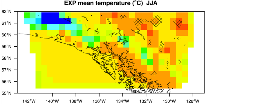
According to the CRU data (Figure 2), mean temperatures were highest over the Chatham Strait (see Figure 1 for location), its adjacent land and locally in Canada (>12˚C), intermediate along most of the Gulf of Alaska (7.5˚C - 12˚C), and lowest over the glaciers of the St. Elias Mountains (<3˚C).
Judged by the CRU data EXP performed quite similarly to CON in all months and JJA, and captured those climatological features acceptably (Figure 2). Temperature climatology differed insignificantly from the CRU temperatures. Like CON, EXP showed small negative biases in mean 2m temperatures over land, i.e. WRF- chem was slightly too cold. In both simulations, biases were lowest over glaciers and largest along the coast. Except in some areas over Canada, EXP derived 2m temperature means fell within one standard deviation of the CRU data. Similar was true for CON. However, EXP performed slightly weaker in capturing internanual variability than CON as is indicated by the larger area with temperature outsides the range of one standard deviation of the observations (hashed area in Figure 2). Furthermore, EXP more strongly underestimated temperatures over the fjords than CON did.

Table 1. Comparison of JJA skill scores as obtained for climatology determined by downscaling of CESM (EXP) and WRF- chem simulations driven with analysis data (CON) with gridded climatology from observations (OBS). OBS stands for the CRU (2m air temperature, 2m relative humidity, accumulated precipitation; land only) and SBW (10m wind speed; ocean only) data. Bias is simulated minus observed climatology.
Table 2. JJA skill scores as obtained for 2m air temperature, 2m relative humidity, and 10m wind speed climatology determined from downscaled CESM results (EXP) and WRF-chem simulations driven with analysis data (CON). All available data from the 42 sites (OBS) were used in the calculation of the skill scores. Bias is simulated minus observed climatology. Data for individual months look similar to those for JJA (therefore not listed). Standard deviation relates to the sites among each other over all seven years.
 (a)
(a)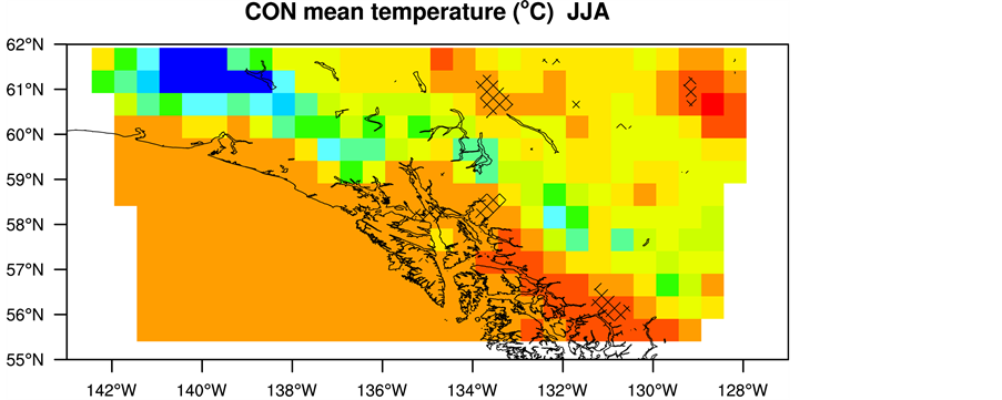 (b)
(b)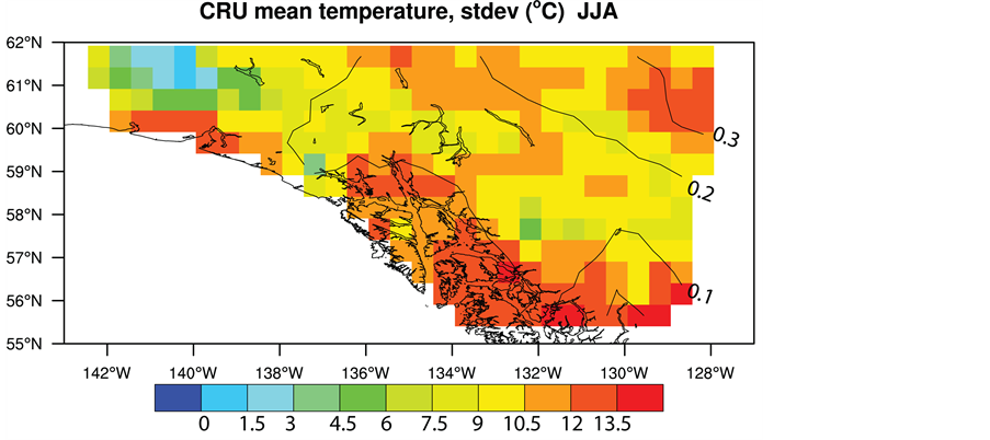 (c)
(c)
Figure 2. Comparison of JJA mean 2m air temperature as obtained by (a) EXP, (b) CON, and (c) according to the CRU data. The contour lines in (c) are the observed standard deviations at 0.1˚C increment. The hashed areas in (a) and (b) indicate where the obtained climatological mean failed to fall within one standard deviation of the observed climatology. CRU data are land only.
Over land, EXP reproduced the climatology of mean temperatures with slightly less accuracy than CON at the southern, eastern and northern boundary of the domain. Since the FNL data are based on observations, they indirectly import information about the response of the meteorological fields to the real upwind landscape into the domain at the inflow boundaries. In CESM, a mosaic approach considered subgrid-scale heterogeneity of land- cover. The landscape in the CESM grid-cell differs from that at the same location in nature by being smoother and less heterogeneous [62] [63] . Thus, when downscaling CESM, the atmospheric response imported over the boundaries is that to a smoother landscape.
According to the CRU data, the interannual variability in mean 2m temperatures was less than 1˚C over land (Figure 2). Over Canada, EXP overestimated the interannual variability locally up to 2.6˚C in June. As expected from theory, both EXP and CON provided smaller interannual variability over the Pacific and coastal areas than inland in all months and JJA. The locally notable discrepancy between WRF-chem derived and CRU temperature climatology may be partly related to the interpolation of sparse data with sites being mainly in valleys or at low elevation (cf. [24] ). The climatology of means and standard deviation derived from EXP (and CON) considered WRF-chem values of all elevations within the 0.5˚ × 0.5˚ area represented by a CRU grid-cell. The locally higher June interannual variability in EXP (and CON) compared to the CRU data suggests that snow at high elevation may have led to increased interannual variability. When interpolating observations from a network favoring valley locations interannual variability in snowline occurring at comparatively higher elevations cannot be captured.
The EXP overall RMSE was the same as in CON, while the overall cold bias was slightly higher (Table 1). The overall EXP and CON 2m temperature means were closer to each other than to the mean determined from the CRU data.
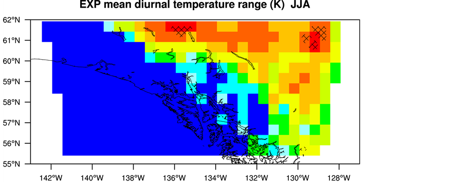
According to the CRU data, the mean JJA diurnal temperature range (DTR) was smallest over the coastal fjords (>4.8˚C) and gradually increased with distance from the ocean to up to 14˚C or more (Figure 3). For all three months, EXP captured this distribution very well and better than CON. EXP dampened the mean DTR slightly less than CON did. On average over JJA, and in July and August, EXP (like CON) broadly captured the areas of largest DTR. Like CON, EXP underestimates the DTR up to 5˚C along the coasts in all months and JJA. EXP well captured the DTR inland over Canada with close to zero biases. Here and along the coasts, EXP outperformed CON. These findings suggest that (1) the bias was rather due to the prescribed SSTs than the lateral forcing data, (2) downscaling with WRF-chem produced better DTR inland than along the coasts in all summer months, and (3) EXP results were of similar quality than we know from forecasts with analysis data.
In EXP, in all months and JJA, the mean DTR changed at the western and eastern domain boundary by about 1˚C - 3˚C absolute as compared to the values slightly more to the east and west, respectively (Figure 3). This feature neither existed in CON nor in the CRU climatology. Therefore, it must be due to the forcing at the lateral boundaries.
The different resolutions cannot be the main reasons as the feature occured on all boundaries in EXP. WRF-chem obtained temperature forcing data of coarser resolution at the western and eastern boundary in EXP than CON (1.25˚ vs. 1˚). The opposite was true for the southern and northern boundary (0.9˚ vs. 1˚). Despite the finer latitudinal resolution of the CESM forcing data at the southern and northern boundaries, CON outperformed EXP here too (Figure 3). These findings can be explained as follows: FNL data base on observations. These observations indirectly included real world signals related to the SST and/or complex terrain in the upwind of the model domain. Consequently, in CON, better information about the conditions outside of the domain was imported over the inflow boundaries than in EXP. Furthermore, in the ABL, temperature advection over the western and eastern boundary was stronger in the CESM than FNL data.
The evaluation by the 42 sites climatology (Figure 4) revealed that EXP (CON) underestimated the monthly mean 2m temperature by 1.6˚C (1˚C). EXP (CON) underestimated the monthly mean diurnal course of 2m temperatures less than 2.2˚C (1.9˚C) in all months, and 2.1˚C (1.6˚C) for JJA. These biases fall within the range found for WRF studies in hindcast mode (e.g. [64] ). Thus, despite EXP reproducted the temperature climatology with slightly less accuracy than CON, its climatology must be considered as being of similar quality. In both cases, differences were smallest at the land sites. This fact hints at errors in advection and SSTs as potential causes. Both simulations used the same SSTs to restrict differences to the lateral forcing.
The spatial and temporal standard deviation obtained by EXP over all 42 sites was 3.5˚C, i.e. less than found in the observed climatology (Table 2). However, EXP captured this moment slightly better than CON. Consequently, the downscaled local scale climate can be considered as acceptable.
 (a)
(a)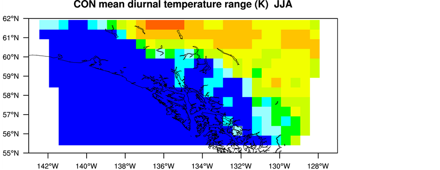 (b)
(b)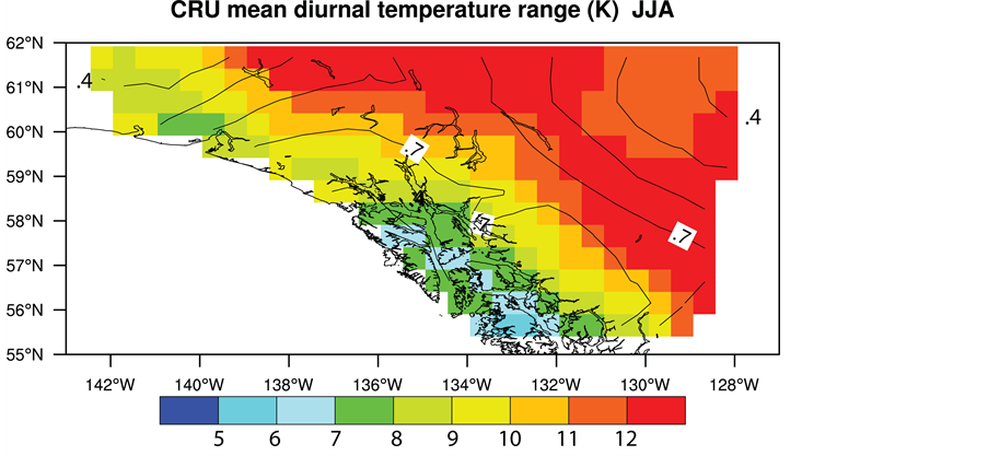 (c)
(c)
Figure 3. Comparison of JJA mean diurnal temperature range as obtained by (a) EXP; (b) CON; and (c) according to the CRU data. The contour lines in (c) are the observed standard deviations at 0.1˚C increment. The hashed areas in (a) and (b) indicate where the obtained climatological mean failed to fall within one standard deviation of the observed climatology. CRU data are land only.

Figure 4. Evaluation of hourly climatology of (upper left to lower right) mean 2m air temperature, 2m relative humidity, 10m wind speed, and 10m wind direction as derived from WRF-chem data with the two different forcings and from hourly observations at the 42 sites (for locations see Figure 1). Data shown are averages over all available data. Curves for individual sites look similar. Note that the time on the x-axis is given with respect to UTC and Alaska Standard Time is UTC-9h. Therefore, the late nighttime minimum temperature occurs in the middle of the plot.
According to the data of the 42 sites, the interannual variability was less than 0.4˚C on average over all sites. EXP provided a nearly twice as high interannual variability of 0.7˚C, but it is the same as obtained by CON. Given that most of the 42 sites are in steep valleys, they frequently may be below the inversions, and hence decoupled from the atmospheric flow at higher levels in the ABL. In the model, however, steep valleys are of subgrid scale and large valleys are smoothed. Thus, the measurements may often represent local mesoscale phenomena that are of subgrid-scale with respect to the model resolution. Consequently, interannual varibility was higher at the grid-cells of the 42 sites in EXP (and CON) than at the actual sites.
Furthermore, the model values represent volume averages, while the observations are point measurements [65] [66] . For all these reasons, following the same argumentation as above, the differences between EXP and observed temperature climatology seem not to be alarming. The quality of EXP produced temperature climatology was similar to that of CON.
The analysis of the site climatology confirmed the results of the evaluation by the CRU data that EXP (like CON) dampened the diurnal cycle in all summer months (Figure 4). The buoy data indicated that this dampening also occurred over water. The forcing governed how the diurnal cycle was dampened. EXP overestimated the mean maximum temperatures in all months, but underestimated the minima. CON well captured the mean temperature minima in all months, but underestimated the mean maxima notably. Thus, we may conclude that the forcing data impacted the overall temperature base state, but parameterizations within the atmospheric part of WRF-chem dampened the DTR.
Averaging over the various surface categories (Figure 5) revealed that in general, EXP provided slightly higher temperatures over land than CON did. In all months, EXP provided distinct differences between the mean 2m temperatures and their diurnal behavior over ocean, land, the coastal area, and Glacier Bay. Over ocean, EXP provided, on average, lower values than CON. These differences increased as summer progressed from about 1.5˚C in June to about 1.8˚C in August. Over Glacier Bay and the coast, temperature differences between EXP and CON were smaller than over the ocean. However, EXP still provided lower temperature means than CON. The prescribed SSTs that were the same in both simulations may be the cause. However, in CON, SSTs were in balance with the atmosphere at the lateral boundaries, while in EXP here, the atmosphere was in balance with the CESM SSTs. This finding indicates that uncertainty in SST may notably affect 2m temperatures over ocean. While EXP and CON provided nearly the same mean temperatures over Glacier Bay in June and August,

Figure 5. Comparison of JJA mean diurnal ranges of 2m air temperature, 2m relative humidity, 10m wind speed, and 10m wind direction climatology (upper left to lower right) as obtained over various surface categories from WRF-chem results when downscaling CESM data (EXP) and when using analysis data as forcing for WRF-chem (CON). In contrast to Figure 4, here only climatologies derived from WRF-chem simulations are shown as too few data or no exist to derive statistically meaningful climatologies from the surface meteorology sites. Note that the y-axes of Figure 4 and Figure 5 differ. Like in Figure 4, time on the x-axis is given with respect to UTC and Alaska Standard Time is UTC-9h.
EXP produced up to 0.5˚C lower mean daytime temperatures in July than CON. Only over land, EXP provided higher mean 2m temperatures than CON.
3.2. Humidity
The discussion of relative humidity (RH) uses absolute values. In general, JJA mean climatology derived from the CRU data showed a decrease of relative humidity from the coast (>90%) inland (60% - 80%). This inland region of low RH was at its largest in June. As summer progressed, RH slightly increased to 70% - 80% nearly everywhere in this region.
In all months, EXP like CON reproduced the spatial and temporal features seen in the CRU data, but with an eastward offset. The distribution of EXP biases and their magnitude were very similar to that of CON. In all months, EXP showed negative biases (−10% to ~0%) over the coastal fjords and glaciers of the St. Elias Mountains. Inland, EXP (like CON) RH biases reached up to ~30% in the north and decreased southwards to below 17%. This means WRF-chem derived RH climatology showed notably and slightly too wet climate in the northern and southern inland areas, respectively.
The spatial offset and overestimation of relative humidity can be related to the differences in terrain height in the model and nature. The comparatively lower orographic barrier in WRF-chem permitted moisture advection farther inland than it actually occurred. The close to zero bias in the fjord landscape indicates that WRF-Chem reproduced relative humidity climatology well over Glacier Bay National Park independent of the forcing.
In all three months, the CRU data showed RH interannual variability of more than 5%, less than 4% and ~3% (absolute) over the continental inland, the fjords and the St. Elias Mountains, respectively. EXP like CON captured this distribution broadly with EXP outperforming CON. Spatial heterogeneity in interannual variability was larger in the WRF-chem derived climatology than the CRU data. However, the low spatial heterogeneity seen in the CRU data may be an artifact from interpolating few observations onto a grid in complex terrain (cf. [24] [52] ). Like CON, EXP underestimated interannual RH variability locally by more than half. In both cases, interannual variability was smaller over the St. Elias Mountains and fjords than according to the CRU derived data. EXP captured the high inland interannual variability of RH in about 50% of the area. CON merely reproduced that here interannual variability exceeded that close to the ocean. This means farther inland, EXP captured interannual variability of relative humidity much better than closer to the ocean and than CON did. Over the fjord landscape, EXP (like CON) derived RH climatology fell within one standard deviation of the observed climatology in all three months and JJA.
For EXP (like CON) RH biases decreased in July and August as compared to June. Nevertheless, RH biases reached still up to 28% locally over the northern inland in August. The overall bias of EXP was 16% in June, 12% in July and August, and 13% for JJA. These overall biases differed insignificantly from those in CON (19%, 14%, 13%, 15%). In EXP (CON), overall June to August and JJA RMSEs were 20%, 17%, 16% and 18% (23%, 18%, 17%, 19%), respectively. The decrease in RMSE and bias over summer means that WRF-chem performed better when low than when high pressure systems governed the synoptic situations.
On average over all sites, EXP overestimated the 42 sites mean relative humidity climatology by 5% for JJA (Table 2). Thus, its performance insignificantly exceeds that of CON that overestimated relative humidity climatology by 7%. EXP captured mean relative humidity excellently at night, when relative humidity was highest (Figure 4), with an average bias less than 1%. On the contray, CON showed a negative bias (−2%). However, both biases fall in the range of current accuracy in measuring RH. Thus, downscaling of CCSM data provided excellent RH climatology for the 42 sites at night. EXP overestimated daytime relative humidity on average less than 11% with lowest overestimation of about 8% in August (Figure 4). This performance is insignificantly better than that of CON (13%, 9%, respectively). On average over all sites, the mean diurnal RH cycles of EXP and CON differed less than 3%, 2%, 2% and 2% in June, July, August, and JJA, respectively.
In the domain, over ocean, coastal areas, Glacier Bay, and land, downscaled climate seemed to be slightly drier than the climate obtained from WRF-chem simulations driven by analysis data (Figure 5). On the mesoscale, under calm wind conditions, relative humidity typically has a diurnal cycle with higher values at night than day. In all months, downscaled relative humidity climatology reproduced this feature quite similar to CON. EXP also captured that the diurnal cycle of RH should be larger over land than ocean as suggested from theory and CON. EXP produced quite similar climatology of the mean diurnal relative humidity range (EXP-CON < 4%) than CON over land and Glacier Bay, with lowest differences in August. The mean relative humidity diurnal cycle was offset entirely towards slightly lower values over the ocean and coast. These findings suggest SSTs as cause rather than differences in forcing.
Overall these findings suggest that when driven with CESM data, WRF-chem derived JJA relative humidity climatology including its diurnal cycle was at least as reliable as that derived from WRF-chem when driven with analysis data (known performance) and even better far inland.
3.3. Precipitations
Precipitation occurrence and amount are among the hardest to predict, especially in mountainous terrain and summer [67] [68] . Here precipitation data are also the hardest to interpolate as gauges are often at low elevation and precipitation increases with height [69] . In summer, sparse networks have difficulties to catch convective precipitation [24] . In most of the Canadian part of the domain, convective precipitation prevails during summer. Thus, caution is needed in trusting the EXP, CON, and gridded data as well. Our analysis assessed the downscaled precipitation compared to known performance with this knowledge in mind.
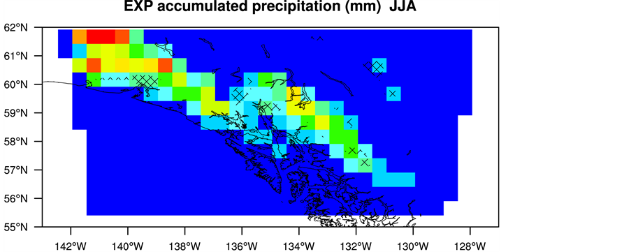
The CRU data report JJA-accumulated precipitation of 225 mm to more than 450 mm in the Coast Mountains, and as low as about 120 mm inlands (Figure 6). In all months, the CRU climatology showed highest accumulated precipitation over the fjord landscape, and the least far inland.
Both simulation-derived climatologies failed capturing the broad distribution and underestimated JJA accumulated precipitation appreciably, but with similar magnitude (Figure 6). Biases were strongest over the Coast Mountains (£350 mm) and lowest over northern British Columbia (<150 mm). Over the backranges independent of the forcing data, WRF-chem simulated the highest accumulated precipitation east of the fjord landscape in all months. This similar behavior suggests that WRF-chem had difficulties in simulating precipitation from orographically forced lifting to its full extend. This shortcoming is well known and common to all grid-models (e.g. [67] ).
In nature, the mountains of the fjord landscape are the first orographic barrier. The mountain ranges in their downwind already face rainshadow effects (Figure 6). WRF-chem, like all numerical weather prediction and air-quality models, used the average terrain height within a grid-cell as representative for the terrain height within the grid-cell. Therefore, any orographic barrier is much lower than in nature. In Southeast Alaska, using an average terrain height leads to a more or less gradual increase of topography from the ocean to the mountain ranges east of the fjord landscape. Consequently, the orographically forced lifting was weaker in the model than real world. This well known model artifact leads to systematic errors in simulated precipitation [67] .
For Southeast Alaska the orographic lifting and orographically forced precipitation in WRF-chem were strongest where in nature, the rainshadow affects climate. Thus, orographic precipitation was produced too far to the East (Figure 6). Consequently, here the largest biases and RMSE occurred, and the climatology of simulated and observed accumulated precipitation differed by more than one standard deviation. Downscaled precipitation (like precipitation predicted using analysis data) was more reliable inland than in the coastal fjord regions. Independent of the forcing data, accumulated precipitation was strongly underestimated in the upwind of the mountain ranges along the Gulf of Alaska. Negative biases occurred in all months, but were lowest in August, the wettest summer month.
Additional reasons for the strong biases may be related to the network’s representing mostly valley sites, its low density and the interpolation [24] [52] [69] . Precipitation even can differ strongly in the same valley depending on elevation and orientation to the main wind direction [70] .
Like CON, EXP captured that monthly accumulted precipiation increased from June to August, and failed capturing the increase to its full degree. For instance, June mean accumulated precipitation of EXP (and CON) underestimated that of CRU slightly in the northern part of the domain, and by more than half over the southern fjords, and their adjacent mountains. In these locations, the biases between simulated and observed accumulated precipitation climatology grew from June towards August in EXP (and CON). In all months, the horizontal distribution of EXP accumulated precipitation biases marginally differed from those of CON. Overall the EXP mean accumulated JJA precipitation was only about half of what it should be according to the CRU data, and even less than half in the case of CON (Table 1).
These findings mean that EXP produced precipitation climatology of similar quality than CON (known performance). However, this underestimation and eastward shift of precipitation could notably affect the simulation of aerosol concentrations, wet and dry deposition.
 (a)
(a) (b)
(b)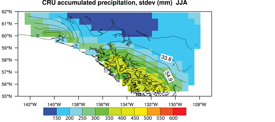 (c)
(c)
Figure 6. Comparison of JJA accumulated precipitation climatology as obtained by (a) EXP; (b) CON; and (c) according to the CRU data. The contour lines in (c) are the observed standard deviations. The hashed areas in (a) and (b) indicate where the obtained climatological mean failed to fall within one standard deviation of the observed climatology. Note that CRU data are land only.
According to the CRU data, the interannual variability of accumulated JJA precipitation is less than 22 mm inland and locally about 88 mm over the glaciers of the St. Elias and Coastal Mountains (Figure 6). Here, the high JJA interannual variability can be associated with slight shifts in the storm-tracks, and lee and luv effects. Inland precipitation mainly stems from convection, which is random, and has low interannual variability.
The CRU distributions of interannual variability were similar in all months, and showed increasing interannual variability as summer progressed. Like CON, EXP captured this trend, but not to the full extend. Like CON, EXP notably underestimated the magnitude of interannual variability in accumulated precipitation climatology and its horizontal heterogeneity. EXP failed to capture the interannual variability over the fjord landscape, but caught broadly the spatial distribution of high and low interannual variability downwind of the Coast Mountains. However, the interannual variabilities were notably (locally nearly eight times) lower than reported in the CRU data. In contrast to EXP, CON failed capturing the spatial distribution of interannual precipitation variability in all months.
The CRU data indicated 47 to 55 wet days in JJA. Like CON, EXP captured the landward decrease in wet days, mislocated the minimum, its horizontal extend, and overestimated the number of wet days. Both provided climatologies with more than 81 wet days nearly everywhere for JJA. This means that WRF-chem predicted precipitation with low amounts too often independent of the used forcing. EXP slightly less overestimated the number of wet days due to its slightly warmer conditions than CON. Some of the overestimation of wet days may be attributed to the cold bias.
The CRU data showed the highest interannual variability in JJA wet days (<7 d) over Canada and the lowest along the coast (~2.5 d). EXP (like CON) failed capturing the distributions of wet-day interannual variability in all months and JJA. However, both showed similar spatial heterogeneity in interannual variability of wet days among each other. Nevertheless, EXP (and CON) interannual variability of wet days remained lower or equal to 9 d for JJA. The EXP and CON results differed due to the different forcing that meant different vertical temperature gradients and stability. The much larger differences between EXP and CRU (or CON and CRU) than between EXP and CON may also be partly associated with the density of the observational network and site locations. In Southeast Alaska, data availability for creating the CRU data was sparse, and screwed towards valleys and easy accessible locations.
Unfortunately, the 42 sites had no precipitation data. Overall the above findings suggest that when downscaling CESM data with WRF-chem in Southeast Alaska, errors in simulated air quality related to precipitation will be similar to those known from WRF-chem driven with analysis data.
3.4. Wind
Reconstruction of wind speeds from satellite observations is possible over water; typically, such reconstructed wind speeds show differences to buoy-recorded wind speeds of less than 0.6 m/s with a standard deviation of about 2.5 m/s [71] .
Over the ocean, the BSW data showed a horizontal gradient in 10m wind speeds from 4.75 m/s in the Gulf of Alaska to more than 5.5 m/s in the southern domain (Figure 7). In JJA, June, and July, the EXP derived climatology showed no such north-south gradient. The same was true for CON. Both EXP and CON captured the north-south gradient of increasing wind speeds over the ocean in August and the board picture in JJA. Both EXP (and CON) underestimated wind speeds over water by 1 m/s and nearly 4 m/s in the north and south, respectively. EXP provided slightly higher wind speeds, and marginally better wind climatology than CON.
Over open ocean, EXP (like CON) wind-speed biases were less than 1 m/s, while along the coast they were typically less than 2 m/s. Here, the similarity of the EXP and CON bias pattern suggests systematic errors in WRF-chem due to discrepancies in the coast-line in the model and nature as causes rather than the forcing data. On average, the EXP negative bias was only 0.5 m/s, i.e. more than about half of CON’s (Table 1). The RMSE of EXP was 0.4 m/s like in CON.
Unfortunately, no gridded wind data was available over land. Here the mean 10m wind speeds derived from EXP exceeded those from CON locally by more than 2 m/s, especially over the St. Elias Mountains (Figure 7). Typically the CESM data provided relatively higher wind speeds at the lateral boundaries due to the smoother terrain in CESM than nature. The analysis data based on various observational data, i.e. signals related to rough ocean surface or complex terrain were included indirectly through the observations, at least, to a certain degree.
 (a)
(a)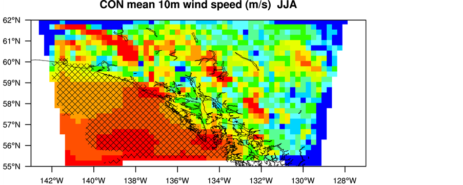 (b)
(b)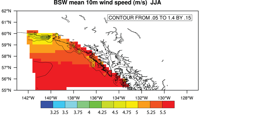 (c)
(c)
Figure 7. Comparison of JJA mean 10m wind-speed climatology as obtained by (a) EXP; (b) CON; and (c) according to the BSW data. The contour lines in (c) are the observed standard deviations. The hashed areas in (a) and (b) indicate where the obtained climatological mean failed to fall within one standard deviation of the observed climatology. Note that BSW data are ocean only.
On JJA mean and in each summer month, the BSW data showed high interannual variability in mean 10m wind speeds ranging from around 0.4 m/s to locally more than 1.4 m/s along the coast (Figure 7). Accoding to the BSW data, interannual variability in mean wind speed was highest over the fjords, locally up to 2.2 m/s. In EXP (like CON) wind climatology failed to fall within one standard deviation of the observations.
EXP (like CON) captured the interannual wind-speed variability (<1 m/s) acceptably in most places along the coast. According to the BSW data, interannual variability decreased over the ocean from north (<1.4 m/s) to south (~0.4 m/s). EXP (like CON) failed reproducing these distributions in all three months everywhere. During this time, EXP provided interannual variabilities between 0.7 m/s and nearly 1.2 m/s in the northern Gulf of Alaska. Here, CON’s interannual variability ranged between 0.7 m/s and 1 m/s. Even though both underestimated interannual variability, downscaled climatology reproduced the interannual variability in wind speed slightly better than that derived from WRF-chem driven by analysis data. EXP (like CON) captured the interannual wind-speed variability in the southwestern Gulf of Alaska.
These findings suggest the surface layer, roughness length and/or ABL parameterizations as potential error causes for the underestimated wind speeds over the ocean. Given the low observed interannal variability in mean wind speeds, the uncertainty in satellite-derived wind speeds, the insignificant differences between EXP and CON, and that the biases are of the order of the accuracy in reconstructed wind speeds one has to conclude (1) that downscaled wind speeds acceptably reproduce observed wind-speed climatology over the ocean and (2) that they were of similar quality than known performance.
Both EXP and CON overestimated the 42 sites monthly mean 10m wind speeds (Figure 4) by less than 2.17 m/s and 1.85 m/s, respectively. In JJA, EXP had negligibly lower bias in seasonal mean 10m wind speeds than CON (1.70 m/s vs. 1.72 m/s). This means that downscaling of CESM data provides reliable summer wind climatology in Southeast Alaska. June and August wind climatology from downscaling were notably weaker (biases of 2.17 m/s, 2.02 m/s vs. 1.59 m/s, 1.85 m/s, respectively), while the July wind-climatology bias broadly agreed with that of CON (1.79 m/s vs. 1.61 m/s). These findings suggest that seasonal wind climatology of EXP is reliable and in the ballpark of current quality of 10m wind-speed forecast with analysis data (e.g. CON) and other studies using analysis or reanalysis forcing (e.g. [30] [72] ).
On average over all seven years and 42 sites, EXP (like CON) reproduced the mean diurnal cycle of wind speed with higher values at daytime than nighttime (Figure 4). EXP overestimated monthly means of hourly 10m wind speeds throughout the entire diurnal cycle by up to 2.20 m/s. EXP performed slightly better than CON, which overestimated monthly means of hourly 10m wind speeds by up to 2.47 m/s. Overestimation by EXP (CON) was largest in June (August). This means the different forcings can affect the time of best performance also on the sub-diurnal scale.
Nighttime overestimation exceeded that at daytime meaning a dampening of the diurnal cycle of wind speed. This fact suggests that WRF-chem had difficulty to capture the full strength of nighttime stability. The surface layer and/or ABL parameterizations are potential causes [73] . Except in August, EXP always provided slightly higher 10m wind speeds than CON. This general overestimation of 10m wind speed agrees with results from previous studies on WRF’s performance in reproducing inversions and/or the wind field under stagnant or calm wind conditions [19] [73] [74] .
The diurnal cycle of observed 10m wind-speed climatology of June and JJA were quite similar making June a good representative of summer 10m wind speeds in Southeast Alaska (Figure 4). WRF-chem reproduced this feature well with both forcings. The EXP and CON derived 10m wind-speed climatology differed less among each other than they differed from the climatology gained from the 42 sites. This finding suggests that systematic errors in 10m wind speed due to local subgrid-scale features (channeling, wind shadows, etc.), misrepresentation of the landscape, and parameterizations in WRF-chem exceeded the differences due to the forcing data.
Interestingly, the onset of wind-direction changes occurred earlier in nature than in the model. Obviously, subgrid-scale local differences in insolation and/or topography play a role. The former is supported by the fact that the change occurred earlier in EXP than in CON. EXP and CON differed in relative humidity and hence cloudiness and insolation. Unfortunately, too few (in space and time) shortwave-radiation data were available for a meaningful statistic. Thus, a further investigation for the temporal offsets has to be postponed to the future.
The average interannual variability was 0.6 m/s at the 42 sites. Here EXP underestimated the interannual variability as strongly as 0.22 m/s, on average. Interannual variability of EXP wind speeds marginally differed from the 0.28 m/s obtained by CON. This about three times and twice lower internannual variability of the WRF-chem derived climatology resulted from the discretization. In nature, the sites are in steep valleys. Here, slight shifts of wind directions were decisive whether or not a channeling effect occurred in a valley. In the model, steep valleys are of subgrid-scale. Thus, slight shifts of wind direction, even when captured by the model, do not result into acceleration or deceleration of 10m wind speed as the topography within the grid-cell is flat. Recall that topography only differed between adjacent grid-cells.
In both WRF-chem derived climatologies, mean 10m wind speeds increased as summer progressed due to the increase in storms. Generally, over land, ocean, coastal areas and Glacier Bay the EXP and CON mean diurnal cycles of 10m wind speeds were nearly the same, but EXP mean wind speeds exceeded those of CON on average (Figure 5). The near-surface wind forcing provided by the CESM data at the lateral boundaries was stronger than that provided by the analysis data, especially over land. These differences in forcing data were due to the fact that the analysis included the real surface impact on wind speeds. CESM used a mosaic approach for the various plant-functional types [75] . Any mosaic approach simplifies and smoothens the heterogeneity of the landscape [61] [76] , for which the likelihood for overestimation of wind speed increases.
Over the ocean, both CESM and WRF-chem calculated surface-roughness lengths depending on grid-volume mean wind speed. The relatively coarse horizontal resolution of CESM means smoothening high roughnesses due to waves that may exist at fine resolution. Thus, the CESM forcing data provided enhanced wind speeds to WRF-chem at the lateral boundaries as compared to the analysis data. Comparison of the EXP obtained 10m wind speeds over land and ocean revealed that downscaling mitigated the enhanced wind forcing of CESM over the ocean as the air moved towards the center of the domain. In EXP, the increased wind forcing at the lateral boundaries meant increased ocean-surface roughness in WRF-chem, which counteracted wind speed. Probably, the analysis data may also have provided stronger wind fields than existed in nature because of the limited data availability over water, and the gridding procedures (cf. [24] ). Since the analysis data based on observations small-scale impacts of roughness were indirectly included to a certain degree despite of the relatively coarse resolution. The low data density explains some of the systematic differences found in this and many other studies between simulated and observed wind fields [74] [77] .
Both WRF-chem derived climatologies showed small differences between nighttime and daytime mean wind directions over the domain, land, and ocean, and comparatively wider diurnal cycles over coastal areas and Glacier Bay (Figure 5). In all summer months, the mean hourly wind-direction climatology of EXP and CON differed greater at night than day, and the strongest (up to ~60˚) over water at night. The former is partly related to differences in wind components at the lateral boundaries, and partly to differences in surface roughness. Since in WRF-chem, surface roughness over water depends on wind speed, wind-speed differences at the lateral boundaries propagated into differences in surface roughnesses, and wind direction in the domain. Over land, ocean, and the coastal area winds showed slightly more northern components in EXP than CON.
In Glacier Bay, however, at night, on average, winds came with slightly western and eastern components in EXP and CON, respectively. Furthermore, in Glacier Bay, EXP and CON wind-direction climatology showed a slight temporal offset. In Glacier Bay, the diurnal cycle of wind direction was very distinct (>70˚) in EXP like in CON (Figure 5). Distinct differences between day and night were expected because of frequently occurring nighttime inversions, mountain-valley circulations and circulations in and out of the bay. The downscaling captured effects due to these features similar to CON.
The coastal wind-direction climatology of EXP showed differences between day and night of ~50˚ indicating that the downscaling captured occasionally occurring sea and/or land breeze systems. EXP captured these mesoscale features slightly, but insignificantly weaker than CON.
Overall downscaling of CESM data by WRF-chem provided acceptable wind climatology. According to the evaluation downscaled wind-speed fields had similar shortcomings, and only marginally lower quality as we know from WRF-chem driven by analysis.
Typically, the differences between the EXP and CON wind climatology were less than those between them and the observed climatology. Independent of the forcing, 10m wind-speed climatology was overestimated throughout the entire diurnal cycle. The wind climatologies of EXP and CON showed positive bias, and WRF- chem produced only marginally (insignificant) lower quality 10m wind-speed climatology when forced with CESM than when forced with analysis data. However, both the EXP and CON derived wind climatology failed to fall within one standard deviation of the observations over large areas of the ocean. Given the low observed interannal variability in mean wind speed, the uncertainty in satellite-derived wind speeds, and the non-significant differences over land and with respect to different mesoscale environments, we may conclude that downscaling of CESM data by WRF-chem can provide realistic regional results with similar fidelity as known for WRF- chem forecasts with analysis with respect to the wind fields.
4. Conclusions
Assessment of future summer air quality and impacts of various alternative/combined management decisions regarding cruise-ship traffic in Glacier Bay National Park requires reliable regional air-quality simulations of future climate. This study examined the performance of WRF-chem in downscaling CESM data (experiment, EXP) in comparison to WRF-chem simulations forced with analysis data (control, CON). The latter represents the “known performance” of modern air-quality models. The climatology derived therefrom served as a relative benchmark for Southeast Alaska in this study. In addition, the climatologies derived from the downscaled CESM data were evaluated by gridded climatology of meteorological surface observations from the CRU and blended sea-wind datasets, and climatologies of 42 sites. This strategy permitted assessment of the produced climatologies at various spatial and temporal scales. Unfortunately, in the region of Glacier Bay, no chemical concentration data existed for assessement of the performance in capturing air quality. Thus, this study focused on EXP’s performance in reproducing climatology of temperature, relative humidity, precipitation, and wind as errors in these quantities may propagate into the projected chemical fields (e.g. [19] [78] ).
Summer biases (EXP vs. CRU or BSW) in EXP climatology of 2m air temperature, diurnal temperature range, relative humidity and accumulated precipitation over land and 10m wind speed and direction over ocean amounted 1.1 K, −4.9 K, 13%, −110 mm, −3.8 m/s and 46˚, respectively. This performance was of similar accuracy as that of CON (−0.7 K, −5.3 K, 15%, −120 mm, −4 m/s, 46˚), i.e. state-of-the-art.
Based on the 42 sites EXP showed overall JJA biases in 2m temperature, relative humidity and wind speed over land and ocean of −1.1 K, 5%, and 1.78 m/s, respectively. These biases are similar to those gained from WRF-chem forecasts with analysis data (−1.6 K, 7%, 1.36 m/s). Unfortunately, the tendency of WRF-chem to overestimate low wind speeds is slightly larger in EXP than CON. However, given the complex topography the wind-speed biases are less than one standard deviation (Table 2).
The skill scores based on the hourly data of the 42 sites confirm the findings of the assessment by the gridded data over areas covered by them. Typically, the differences between the EXP and CON climatologies were less than those between them and the observed climatologies. The latter fact leads to the conclusion that downscaling of CESM data by WRF-chem provided results of similar quality than we know from WRF-chem forecasts with analysis data.
Buoys and land sites showed similar scores. Thus, one may conclude that the downscaled meteorological quantities over the ocean (land) not covered by the gridded CRU (BSW) data showed similar quality as found over the land (ocean) covered by them.
Some discrepancies between the downscaled and satellite derived wind speeds may be attributable to mixed pixels and uncertainty in the retrivial algorithm [79] . Some discrepancies between the climatology produced from downscaled CSEM data and the observations can be attributed to sites being mostly in valleys close to settlements, and the low network density over Canada, and in case of the CRU data to the interpolation of sparse data in complex terrain. In valleys, the observations may strongly reflect very local features that are not representative for the area of the grid-cell. For instance, in Southeast Alaska, locations being in the rainshadow of a mountain barrier receive typically less precipitation than those in the leewardside of the next higher mountain barrier; and typically 2m air temperatures are lowest over north and highest over south slopes [57] .
Some discrepancies stem from discretization and observational techiques at meteorology sites. The observations are point measurements, while the downscaled 3D (2D) field quantities are volume (surface) averages over a flat area at the mean terrain height of the grid-cell. Finally, over land chanelling effects are of subgrid-scale and may yield systematic errors due to the discretization of the terrain. However, these uncertainties apply for CON and other air-quality models as well.
The comparison of EXP with CON revelead some model related shortcomings that occurred independent of the lateral forcing data. For instance, EXP and CON showed very similar dampening of mean DTRs everywhere in the domain about one or two increments away from the lateral boundaries. This means the DTR dampening resulted from the parameterizations of the ABL, surface, and/or radiation. Independent of the forcing, the WRF-chem-derived climate overestimated the interannual temperature variability as compared to the CRU data and the 42 sites, but was of similar magnitude in EXP and CON. This behavior can be partly explained by the sites’ being mostly located in steep valleys where local channeling effects and inversions occur. Steep valleys were of subgrid-scale with respect to the resolution of WRF-chem in this study. The representation of topography in WRF-chem caused the underestimation of interannual relative humidity variability over the fjords and St. Elias Mountains, which also occured for both forcings.
The study showed that the forcing data may occassionally compensate—to a small degree—model related errors. Indeed, downscling of CESM data produced a better distribution of wet-day climatology than that obtained when using analysis data as forcing, but for the wrong reasons. The too high number of wet days in EXP and CON, in general, was related to the cloud parameterizations and cold bias. The slightly warmer atmosphere of EXP meant that atmospheric conditions were farther away from saturation than in CON, and the partititing between the warm and cold paths of precipitation formation was shifted to the less efficient warm path. Despite WRF-chem failed capturing the precipitation distribution in great part due to the discretization of topography, the downscaled precipitation climatology was at least of similar quality than current forecasts in Southeast Alaska.
The study revealed sensitivities, and where results were more reliable. Errors in downscaled temperature climatogy and differences between EXP and CON climatologies were higher over coastal than inland areas. This meant that uncertainty in SSTs strongly affected the accuracy of 2m temperatures along the coast and over the ocean in Southeast Alaska. Downscaled climate was most reliable farther inland in areas still far enough away from the lateral boundaries. Interannual variability of wind speeds was best captured in the fjords along the coast.
The study revealed that when downscaling CESM data, a larger domain should be used and/or more data along the lateral boundaries should be discarded form the analysis than it is typically done in regional air-quality forecasts. Analysis data, namely, base on assimilated observations, and inherit fine scale signals. Consequently, even though the analysis data provided the lateral boundary conditions at 1˚ × 1˚ the fields of inflow quantities adapted relatively fast to the finer spatial resolution in the model domain. On the contray, the CESM data were in balance with the topography 0.9˚ × 1.25˚ latitudinal and longitudinal grid of CESM. Therefore, WRF-chem needed more time to adapt to the finer resolution when CESM data were downscaled than with analysis data as forcing. In other words, the inflowing field quantities travelled farther into the domain until they achieved an equilibrium that was consistent with the conditions in the model domain.
The forcing influenced the overall temperature base state in the domain beyond the five lateral grid-cells that were discarded from analysis already. The EXP and CON mean temperatures differed due to the different temperature advection at the lateral boundaries. Obviously, the atmosphere has “memory” of upwind surface conditions via the temperatures in the ABL. This memory was introduced in the regional domain at the inflow boundaries.
The downscaled fields of temperature, diurnal temperature range, wind speed, and relative humidity captured the expected mesoscale responses to regional differences. EXP’s responses were of similar magnitude with those of CON. For instance, downscaling correctly produced increasing DTR land inwards. WRF-chem downscaling also resolved the flow pattern along the coast and in large fjords like Glacier Bay acceptably.
Based on this study we can conclude that the found differences should not yield major difficulties in applying CESM driven regional climate simulations to project air quality over Glacier Bay National Park in summer. We further conclude that downscaling CESM with WRF-chem can provide realistic data for assessment of future air quality within similar uncertainty range than today’s air-quality forecasts driven with analysis data if the emissions and their changes are well understood and assumed realistically.
Overall, the study showed that when driven by CESM data WRF-chem provided climatology of similar (read sometimes marginally weaker/better) quality for Southeast Alaska as WRF-chem did in forecast mode when forced with analysis data. When driven with CESM data WRF-chem reproduced the diurnal cycle of relative humidity climatology with similar accuracy as compared to when forced with analysis data meaning downscaled relative humidity data were at least as reliable as known performance from WRF-chem forecasts with analysis data for Southeast Alaska. In the fjords along the coast, EXP produced similar interannual variability in wind- speed climatology than CON. Downscaling CESM data produced precipitation information (accumulated precipitation, number of wet days, interannual variability, distributions) that was not any worse than is currently achieved in forecasts with analysis data for Southeast Alaska.
Thus, we may conclude that for Southeast Alaska the seven year climatology derived from WRF-chem driven with CESM data provided a comparable thermodynamic and dynamic state than when driven with analysis data. Being aware of current discrepancies in air-quality model results driven by analysis data will be keys to assess downscaled future air quality for this area.
Acknowledgements
The authors thank M.K. Butwin, U.S. Bhatt, G. Kramm, D. PaiMazumder and the anonymous reviewers for fruitful discussions, J. Stickel for additional station data, the University of Alaska Fairbanks’ Geophysical Institute’s supercomupting center for computational and the National Parks Service for financial support (contract P11AT30883/P11AC90465).
References
- Mölders, N., Gende, S. and Pirhalla, M.A. (2013) Assessment of Cruise-Ship Activity Influences on Emissions, Air Quality, and Visibility in Glacier Bay National Park. Atmospheric Pollution Research, 4, 435-445. http://dx.doi.org/10.5094/APR.2013.050
- Mölders, N. and Kramm, G. (2014) Lectures in Meteorology. Springer, Heidelberg, 591.
- Seinfeld, J.H. and Pandis, S.N. (1997) Atmospheric Chemistry and Physics, from Air Pollution to Climate Change. Wiley, New York.
- Real, E. and Sartelet, K. (2011) Modeling of Photolysis Rates over Europe: Impact on Chemical Gaseous Species and Aerosols. Atmosphere Chemistry Physics, 11, 1711-1727. http://dx.doi.org/10.5194/acp-11-1711-2011
- Zhang, Y., Hu, X.M., Leung, L.R. and Gustafson, W.I. (2008) Impacts of Regional Climate Change on Biogenic Emissions and Air Quality. Journal of Geophysical Research: Atmospheres, 113, Published Online. http://dx.doi.org/10.1029/2008JD009965
- Spracklen, D.V., Mickley, L.J., Logan, J.A., Hudman, R.C., Yevich, R., Flannigan, M.D. and Westerling, A.L. (2009) Impacts of Climate Change from 2000 to 2050 on Wildfire Activity and Carbonaceous Aerosol Concentrations in the Western United States. Journal of Geophysical Research: Atmospheres, 114, Published Online. http://dx.doi.org/10.1029/2008JD010966
- Fang, Y., Fiore, A.M., Horowitz, L.W., Gnanadesikan, A., Held, I., Chen, G., Vecchi, G. and Levy, H. (2011) The Impacts of Changing Transport and Precipitation on Pollutant Distributions in a Future Climate. Journal of Geophysical Research: Atmospheres, 116, Published Online. http://dx.doi.org/10.1029/2011JD015642
- Menut, L., Tripathi, O., Colette, A., Vautard, R., Flaounas, E. and Bessagnet, B. (2013) Evaluation of Regional Climate Simulations for Air Quality Modelling Purposes. Climate Dynamics, 40, 2515-2533. http://dx.doi.org/10.1007/s00382-012-1345-9
- McKeen, S., Grell, G., Peckham, S., Wilczak, J., Djalalova, I., Hsie, E.Y., Frost, G., Peischl, J., Schwarz, J., Spackman, R., Holloway, J., De Gouw, J., Warneke, C., Gong, W., Bouchet, V., Gaudreault, S., Racine, J., Mchenry, J., McQueen, J., Lee, P., Tang, Y., Carmichael, G.R. and Mathur, R. (2009) An Evaluation of Real-Time Air Quality Forecasts and Their Urban Emissions over Eastern Texas during the Summer of 2006 Second Texas Air Quality Study Field Study. Journal of Geophysical Research: Atmospheres, 114, Published Online. http://dx.doi.org/10.1029/2008JD011697
- D’Allura, A., Kulkarni, S., Carmichael, G.R., Finardi, S., Adhikary, B., Wei, C., Streets, D., Zhang, Q., Pierce, R.B., Al-Saadi, J.A., Diskin, G. and Wennberg, P. (2011) Meteorological and Air Quality Forecasting Using the WRF- STEM Model During the 2008 ARCATS Field Campaign. Atmospheric Environment, 45, 6901-6910. http://dx.doi.org/10.1016/j.atmosenv.2011.02.073
- Pierce, T., Hogrefe, C., Rao, S.T., Porter, P.S. and Ku, J.Y. (2010) Dynamic Evaluation of a Regional Air Quality Mo- del: Assessing the Emissions-Induced Weekly Ozone Cycle. Atmospheric Environment, 44, 3583-3596. http://dx.doi.org/10.1016/j.atmosenv.2010.05.046
- Mölders, N., Tran, H.N.Q., Cahill, C.F., Leelasakultum, K. and Tran, T.T. (2012) Assessment of WRF/Chem PM2.5 Forecasts Using Mobile and Fixed Location Data from the Fairbanks, Alaska Winter 2008/09 Field Campaign. Atmospheric Pollution Research, 3, 180-191. http://dx.doi.org/10.5094/APR.2012.018
- Van Loon, M., Vautard, R., Schaap, M., Bergström, R., Bessagnet, B., Brandt, J., Builtjes, P.J.H., Christensen, J.H., Cuvelier, C., Graff, A., Jonson, J.E., Krol, M., Langner, J., Roberts, P., Rouil, L., Stern, R., Tarrasón, L., Thunis, P., Vignati, E., White, L. and Wind, P. (2007) Evaluation of Long-Term Ozone Simulations from Seven Regional Air Quality Models and Their Ensemble. Atmospheric Environment, 41, 2083-2097. http://dx.doi.org/10.1016/j.atmosenv.2006.10.073
- Yu, S., Mathur, R., Schere, K., Kang, D., Pleim, J. and Otte, T.L. (2007) A Detailed Evaluation of the Eta-CMAQ Forecast Model Performance for O3, Its Related Precursors, and Meteorological Parameters During the 2004 ICARTT Study. Journal of Geophysical Research: Atmosphere, 112, Published Online. http://dx.doi.org/10.1029/2006JD007715
- Vivanco, M., Palomino, I., Martín, F., Palacios, M., Jorba, O., Jiménez, P., Baldasano, J. and Azula, O. (2009) An Eva- luation of the Performance of the CHIMERE Model over Spain Using Meteorology from MM5 and WRF Models. Pro- ceeding of Computational Science and Its Applications, Seoul, 29 June-2 July 2009, 107-117.
- Zhang, Y., Dubey, M.K., Olsen, S.C., Zheng, J. and Zhang, R. (2009) Comparisons of WRF/Chem Simulations in Me- xico City with Ground-Based Rama Measurements during the 2006-MILAGRO. Atmosphere Chemistry Physics, 9, 3777-3798. http://dx.doi.org/10.5194/acp-9-3777-2009
- Wu, Q., Wang, Z., Chen, H., Zhou, W. and Wenig, M. (2012) An Evaluation of Air Quality Modeling over the Pearl River Delta during November 2006. Meteorology and Atmospheric Physics, 116, 113-132. http://dx.doi.org/10.1007/s00703-011-0179-z
- Appel, K., Roselle, S., Gilliam, R. and Pleim, J. (2010) Sensitivity of the Community Multiscale Air Quality (CMAQ) Model V4.7 Results for the Eastern United States to MM5 and WRF Meteorological Drivers. Geoscience Model Deve- lopment, 3, 169-188. http://dx.doi.org/10.5194/gmd-3-169-2010
- Mölders, N., Tran, H.N.Q., Quinn, P., Sassen, K., Shaw, G.E. and Kramm, G. (2011) Assessment of WRF/Chem to Capture Sub-Arctic Boundary Layer Characteristics during Low Solar Irradiation Using Radiosonde, Sodar, and Station Data. Atmospheric Pollution Research, 2, 283-299. http://dx.doi.org/10.5094/APR.2011.035
- Vautard, R., Solazzo E, Gilliam, R., Matthias, V., Bianconi, R., Ferreira, J., Geyer, B., Hansen, A., Jericevic, A., Prank, M., Segers, A., Silver, J.D., Werhahn, J., Wolke, R., Rao, S.T. and Galmarini, S. (2012) Evaluation of the Meteorological Forcing Used for the Air Quality Model Evaluation International Initiative (AQMEII) Air Quality Simulations. At- mospheric Environment, 53, 15-37. http://dx.doi.org/10.1016/j.atmosenv.2011.10.065
- Done, J.M., Holland, G.M., Bruyère, C.L., Leung, L.R. and Suzuki-Parker, A. (2013) Modeling High Impact Weather and Climate: Lessons from a Tropical Cyclone Perspective. Climate Change, Published Online. http://dx.doi.org/10.1007/s10584-013-0954-6
- Paeth, H. and Mannig, B. (2013) On the Added Value of Regional Climate Modeling in Climate Change Assessment. Climate Dynamics, 41, 1057-1066. http://dx.doi.org/10.1007/s00382-012-1517-7
- Pfister, G.G., Walters, S., Lamarque, J.F., Fast, J., Barth, M.C., Wong, J., Done, J., Holland, G. and Bruyère, C.L. (2014) Projections of Future Summertime Ozone over the US. Journal of Geophysical Research: Atmosphere, 119, 5559-5582. http://dx.doi.org/10.1002/2013JD020932
- PaiMazumder, D. and Mölders, N. (2009) Theoretical Assessment of Uncertainty in Regional Averages Due to Network Density and Design. Journal of Applied Meteorology and Climatology, 48, 1643-1666. http://dx.doi.org/10.1175/2009JAMC2022.1
- Skamarock, W.C., Klemp, J.B., Dudhia, J., Gill, D.O., Barker, D.M., Duda, M.G., Huang, X.Y., Wang, W. and Powers, J.G. (2008) A Description of the Advanced Research WRF Version 3. NCAR Technical Note, 125p.
- Caldwell, P., Chin, H.N., Bader, D. and Bala, G. (2009) Evaluation of a WRF Dynamical Downscaling Simulation over California. Climatic Change, 95, 499-521. http://dx.doi.org/10.1007/s10584-009-9583-5
- Gao, Y., Fu, J.S., Drake, J.B., Liu, Y. and Lamarque, J.F. (2012) Projected Changes of Extreme Weather Events in the Eastern United States Based on a High Resolution Climate Modeling System. Environmental Research Letters, 7, Article ID: 044025.
- Peckham, S.E., Fast, J., Schmitz, R., Grell, G.A., Gustafson, W.I., Mckeen, S.A., Ghan, S.J., Zaveri, R., Easter, R.C., Barnard, J., Chapman, E., Salzman, M., Barth, M., Pfister, G., Wiedinmyer, C., Hewson, M. and Freitas, S.R. (2011) WRF/Chem Version 3.3 User’s Guide. ESSL Technical Note, p. 96.
- Grell, G.A., Freitas, S.R., Stuefer, M. and Fast, J.D. (2011) Inclusion of Biomass Burning in WRF-Chem: Impact on Wildfires on Weather Forecasts. Atmosphere Chemistry Physics, 11, 5289-5303. http://dx.doi.org/10.5194/acp-11-5289-2011
- Lamarque, J.F., Emmons, L.K., Hess, P.G., Kinnison, D.E., Tilmes, S., Vitt, F., Heald, C.L., Holland, E.A., Lauritzen, P.H., Neu, J., Orlando, J.J., Rasch, P.J. and Tyndall, G.K. (2012) CAM-Chem: Description and Evaluation of Interactive Atmospheric Chemistry in the Community Earth System Model. Geoscience Model Development, 5, 369-411. http://dx.doi.org/10.5194/gmd-5-369-2012
- Meehl, G.A., Washington, W.M., Arblaster, J.M., Hu, A., Teng, H., Kay, J.E., Gettelman, A., Lawrence, D.M., Sanderson, B.M. and Strand, W.G. (2013) Climate Change Projections in CESM1(CAM5) Compared to CCSM4. Journal of Climate, 26, 6287-6308. http://dx.doi.org/10.1175/JCLI-D-12-00572.1
- Hines, K.M. and Bromwich, D.H. (2008) Development and Testing of Polar Weather Research and Forecasting (WRF) Model. Part I: Greenland Ice Sheet Meteorology. Monthly Weather Review, 136, 1971-1989. http://dx.doi.org/10.1175/2007MWR2112.1
- Liu, X.H., Zhang, Y., Olsen, K.M., Wang, W.X., Do, B.A. and Bridgers, G.M. (2010) Responses of Future Air Quality to Emission Controls over North Carolina, Part I: Model Evaluation for Current-Year Simulations. Atmospheric Environment, 44, 2443-2456. http://dx.doi.org/10.1016/j.atmosenv.2010.04.002
- Lindvall, J., Svensson, G. and Hannay, C.E. (2013) Evaluation of Near-Surface Parameters in the Two Versions of the Atmospheric Model in CESM1 Using Flux Station Observations. Journal of Climate, 26, 26-44. http://dx.doi.org/10.1175/JCLI-D-12-00020.1
- Hong, S.Y. and Lim, J.O.J. (2006) The WRF Single-Moment 6-Class Microphysics Scheme (WSM6). Journal Korean Meteorological Society, 42, 129-151.
- Grell, G.A. and Dévényi, D. (2002) A Generalized Approach to Parameterizing Convection. Geophysical Research Letters, 29, 381-384.
- Chou, M.D. and Suarez, M.J. (1994) An Efficient Thermal Infrared Radiation Parameterization for Use in General Circulation Models. NASA Technical Memorandum 104606, 3, 85. https://archive.org/details/nasa_techdoc_19950009331
- Mlawer, E.J., Taubman, S.J., Brown, P.D., Iacono, M.J. and Clough, S.A. (1997) Radiative Transfer for Inhomogeneous Atmospheres: RRTM, a Validated Correlated-K Model for the Longwave. Journal of Geophysical Research, 102D, 16663-16682. http://dx.doi.org/10.1029/97JD00237
- Barnard, J., Fast, J., Paredes-Miranda, G., Arnott, W. and Laskin, A. (2010) Technical Note: Evaluation of the WRF- Chem “Aerosol Chemical to Aerosol Optical Properties” Module Using Data from the Milagro Campaign. Atmospheric Chemistry Physics, 10, 7325-7340. http://dx.doi.org/10.5194/acp-10-7325-2010
- Janjić, Z.I. (2002) Nonsingular Implementation of the Mellor-Yamada Level 2.5 Scheme in the NCEP Meso Model. NCEP Technical Note 437, 61p.
- Chen, F. and Dudhia, J. (2000) Coupling an Advanced Land-Surface / Hydrology Model with the Penn State/NCAR MM5 Modeling System. Part I: Model Description and Implementation. Monthly Weather Review, 129, 569-585. http://dx.doi.org/10.1175/1520-0493(2001)129<0569:CAALSH>2.0.CO;2
- Stockwell, W.R., Middleton, P., Chang, J.S. and Tang, X. (1990) The Second-Generation Regional Acid Deposition Model Chemical Mechanism for Regional Air Quality Modeling. Journal Geophysical Research, 95, 16343-16367. http://dx.doi.org/10.1029/JD095iD10p16343
- Madronich, S. (1987) Photodissociation in the Atmosphere, 1, Actinic Flux and the Effects of Ground Reflections and Clouds. Journal Geophysical Research, 92, 9740-9752. http://dx.doi.org/10.1029/JD092iD08p09740
- Ackermann, I.J., Hass, H., Memmesheimer, M., Ebel, A., Binkowski, F.S. and Shankar, U. (1998) Modal Aerosol Dynamics Model for Europe: Development and First Applications. Atmospheric Environment, 32, 2981-2299. http://dx.doi.org/10.1016/S1352-2310(98)00006-5
- Schell, B., Ackermann, I.J., Hass, H., Binkowski, F.S. and Ebel, A. (2001) Modeling the Formation of Secondary Organic Aerosol within a Comprehensive Air Quality Model System. Journal Geophysical Research, 106, 28275-28293. http://dx.doi.org/10.1029/2001JD000384
- Guenther, A., Hewitt, C., Erickson, D., Fall, R., Geron, C., Graedel, T., Harley, P., Klinger, L., Lerdau, M., Mckay, W., Pierce, T. and Zimmerman, P.R. (1994) A Global Model of Natural Volatile Organic Compound Emissions. Journal Geophysical Research, 100D, 8873-8892.
- NCEP (2000) NCEP FNL Operational Model Global Tropospheric Analyses, Continuing from July 1999. http://dx.doi.org/10.5065/D6M043C6
- Community Climate System Model/Climate and Global Dynamics Division/National Center for Atmospheric Research/University Corporation for Atmospheric Research (2011) NCAR Community Earth System Model, EASM Pro- ject Dataset. NCAR Technical Note. http://dx.doi.org/10.5065/D6TH8JP5
- Meinshausen, M., Smith, S.J., Calvin, K., Daniel, J.S., Kainuma, M.L.T., Lamarque, J.F., Matsumoto, K., Montzka, S.A., Raper, S.C.B., Riahi, K., Thomson, A., Velders, G.J.M. and Vuuren, D.P.P. (2011) The RCP Greenhouse Gas Concentrations and Their Extensions from 1765 to 2300. Climatic Change, 109, 213-241. http://dx.doi.org/10.1007/s10584-011-0156-z
- Keppel-Aleks, G., Randerson, J.T., Lindsay, K., Stephens, B.B., Moore, J.K., Doney, S.C., Thornton, P.E., Mahowald, N.M., Hoffman, F.M., Sweeney, C., Tans, P.P., Wennberg, P.O. and Wofsy, S.C. (2013) Atmospheric Carbon Dioxide Variability in the Community Earth System Model: Evaluation and Transient Dynamics during the Twentieth and Twenty-First Centuries. Journal of Climate, 26, 4447-4475. http://dx.doi.org/10.1175/JCLI-D-12-00589.1
- PaiMazumder, D., Miller, J., Li, Z., Walsh, J.E., Etringer, A., McCreight, J., Zhang, T. and Mölders, N. (2008) Evaluation of Community Climate System Model Soil Temperatures Using Observations from Russia. Theoretical and Applied Climatology, 94, 187-213. http://dx.doi.org/10.1007/s00704-007-0350-0
- Harris, I., Jones, P.D., Osborn, T.J. and Lister, D.H. (2013) Updated High-Resolution Grids of Monthly Climatic Observations—The CRU TS3.10 Dataset. International Journal of Climatology, 34, 623-642.
- Zhang, H.M., Bates, J.J. and Reynolds, R.W. (2006) Assessment of Composite Global Sampling: Sea Surface Wind Speed. Geophysical Research Letters, 33, Published Online. http://dx.doi.org/10.1029/2006GL027086
- Chuang, M.T., Zhang, Y. and Kang, D. (2011) Application of WRF/Chem-Madrid for Real-Time Air Quality Forecasting over the Southeastern United States. Atmospheric Environment, 45, 6241-6250. http://dx.doi.org/10.1016/j.atmosenv.2011.06.071
- Kukkonen, J., Olsson, T., Schultz, D., Baklanov, A., Klein, T., Miranda, A.I., Monteiro, A., Hirtl, M., Tarvainen, V., Boy, M., Peuch, V.H., Poupkou, A., Kioutsioukis, I., Finardi, S., Sofiev, M., Sokhi, R., Lehtinen, K.E.J., Karatzas, K., Jos, R.S., Astitha, M., Kallos, G., Schaap, M., Reimer, E., Jakobs, H. and Eben, K. (2012) A Review of Operational, Regional-Scale, Chemical Weather Forecasting Models in Europe. Atmosphere Chemistry Physics, 12, 1-87. http://dx.doi.org/10.5194/acp-12-1-2012
- Kim, J., Waliser, D.E., Mattmann, C.A., Mearns, L.O., Goodale, C.E., Hart, A.F., Crichton, D.J., Mcginnis, S., Lee, H., Loikith, P.C. and Boustani, M. (2013) Evaluation of the Surface Climatology over the Conterminous United States in the North American Regional Climate Change Assessment Program Hindcast Experiment Using a Regional Climate Model Evaluation System. Journal of Climate, 26, 5698-5715. http://dx.doi.org/10.1175/JCLI-D-12-00452.1
- Shulski, M. and Wendler, G. (2007) The Climate of Alaska. University of Alaska Press, Fairbanks, p. 216.
- Bao, J.W., Michelson, S.A., Persson, P.O.G., Djalalova, I.V. and Wilczak, J.M. (2008) Observed and WRF-Simulated Low-Level Winds in a High-Ozone Episode during the Central California Ozone Study. Journal of Applied Meteorology and Climatology, 47, 2372-2394. http://dx.doi.org/10.1175/2008JAMC1822.1
- Tran, H.N.Q. and Mölders, N. (2011) Investigations on Meteorological Conditions for Elevated PM2.5 in Fairbanks, Alaska. Atmospheric Research, 99, 39-49. http://dx.doi.org/10.1016/j.atmosres.2010.08.028
- Loughner, C.P., Tzortziou, M., Follette-Cook, M., Pickering, K.E., Goldberg, D., Satam, C., Weinheimer, A., Crawford, J.H., Knapp, D.J., Montzka, D.D., Diskin, G.S. and Dickerson, R.R. (2014) Impact of Bay-Breeze Circulations on Surface Air Quality and Boundary Layer Export. Journal of Applied Meteorology and Climatology, 53, 1697-1713. http://dx.doi.org/10.1175/JAMC-D-13-0323.1
- Simpson, C.C., Pearce, H.G., Sturman, A.P. and Zawar-Reza, P. (2013) Verification of WRF Modelled Fire Weather in the 2009-10 New Zealand Fire Season. International Journal of Wildland Fire, 23, 34-45.
- Mölders, N., Raabe, A. and Tetzlaff, G. (1996) A Comparison of Two Strategies on Land Surface Heterogeneity Used in a Mesoscale β Meteorological Model. Tellus, 48, 733-749. http://dx.doi.org/10.1034/j.1600-0870.1996.00012.x
- Giorgi, F. and Avissar, R. (1997) Representation of Heterogeneity Effects in Earth System Modeling: Experience from Land Surface Modeling. Reviews of Geophysics, 35, 413-438. http://dx.doi.org/10.1029/97RG01754
- Hines, K.M., Bromwich, D.H., Bai, L.S., Barlage, M. and Slater, A.G. (2010) Development and Testing of Polar WRF. Part III: Arctic Land. Journal of Climate, 24, 26-48. http://dx.doi.org/10.1175/2010JCLI3460.1
- Jacobson, M.Z. (2007) Fundamentals of Atmospheric Modeling. Cambridge Press, Cambridge.
- Friedrich, K. and Mölders, N. (2000) On the Influence of Surface Heterogeneity on Latent Heat Fluxes and Stratus Pro- perties. Atmospheric Research, 54, 59-85. http://dx.doi.org/10.1016/S0169-8095(99)00050-2
- Smith, S.A., Vosper, S.B. and Field, P.R. (2012) Sensitivity of Orographic Precipitation Enhancement to Horizontal Resolution in the Operational Met Office Weather Forecasts. Meteorological Applications. http://dx.doi.org/10.1002/met.1352
- Ebert, E.E., Damrath, U., Wergen, W. and Baldwin, M.E. (2003) The Assessment of Short-Term Quantitative Precipitation Forecasts. Bulletin of the American Meteorological Society, 84, 481-492. http://dx.doi.org/10.1175/BAMS-84-4-481
- Groisman, P.Y. and Legates, D.R. (1994) The Accuracy of United States Precipitation Data. Bulletin of the American Meteorological Society, 75, 215-227.
- Dingman, S.L. (1994) Physical Hydrology. MacMillan College Publishing Company, New York, 575p.
- Tang, R., Liu, D., Han, G., Ma, Z. and De Young, B. (2014) Reconstructed Wind Fields from Multi-Satellite Observations. Remote Sensing, 6, 2898-2911. http://dx.doi.org/10.3390/rs6042898
- PaiMazumder, D., Henderson, D. and Mölders, N. (2012) Evaluation of WRF-Forecasts over Siberia: Air Mass Formation, Clouds and Precipitation. The Open Atmospheric Sciences Journal, 6, 93-110. http://dx.doi.org/10.2174/1874282301206010093
- Mölders, N. and Kramm, G. (2010) A Case Study on Wintertime Inversions in Interior Alaska with WRF. Atmospheric Research, 95, 314-332. http://dx.doi.org/10.1016/j.atmosres.2009.06.002
- Zhao, Z., Chen, S.H., Kleeman, M.J. and Mahmud, A. (2011) The Impact of Climate Change on Air Quality-Related Meteorological Conditions in California. Part II: Present versus Future Time Simulation Analysis. Journal of Climate, 24, 3362-3376. http://dx.doi.org/10.1175/2010JCLI3850.1
- Lawrence, D.M., Oleson, K.W., Flanner, M.G., Thornton, P.E., Swenson, S.C., Lawrence, P.J., Zeng, X., Yang, X.L., Levis, S., Sakaguchi, K., Bonan, G.B. and Slater, A.G. (2011) Parameterization Improvements and Functional and Structural Advances in Version 4 of the Community Land Model. Journal of Advanced Modeling of Earth Systems, 3, Published Online. http://dx.doi.org/10.1029/2011MS000045
- Avissar, R. and Pielke, R.A. (1989) A Parameterization of Heterogeneous Land Surface for Atmospheric Numerical Models and Its Impact on Regional Meteorology. Monthly Weather Review, 117, 2113-2136. http://dx.doi.org/10.1175/1520-0493(1989)117<2113:APOHLS>2.0.CO;2
- Zhong, S., In, H., Bian, X., Charney, J., Heilman, W. and Potter, B. (2005) Evaluation of Real-Time High Resolution MM5 Predictions over the Great Lakes Region. Weather Forecasting, 20, 63-81. http://dx.doi.org/10.1175/WAF-834.1
- Kinnison, D.E., Brasseur, G.P., Walters, S., Garcia, R.R., Marsh, D.R., Sassi, F., Harvey, V.L., Randall, C.E., Emmons, L., Lamarque, J.F., Hess, P., Orlando, J.J., Tie, X.X., Randel, W., Pan, L.L., Gettelman, A., Granier, C., Diehl, T., Nie- meier, U. and Simmons, A.J. (2007) Sensitivity of Chemical Tracers to Meteorological Parameters in the MOZART-3 Chemical Transport Model. Journal of Geophysical Research: Atmospheres, 112, Published Online. http://dx.doi.org/10.1029/2006JD007879
- Pryor, S.C., Nielsen, M., Barthelmie, R.J. and Mann, J. (2003) Can Satellite Sampling of Offshore Wind Speeds Realistically Represent Wind Speed Distributions? Part II: Quantifying Uncertainties Associated with Distribution Fitting Methods. Journal of Applied Meteorology, 43, 739-750. http://dx.doi.org/10.1175/2096.1