Atmospheric and Climate Sciences
Vol. 2 No. 2 (2012) , Article ID: 18831 , 12 pages DOI:10.4236/acs.2012.22022
A General Purpose Analysis Package
1ISAC-CNR (Institute of Atmospheric Sciences and Climate—National Research Council), Rome, Italy
2 CRATI Scrl, University of Calabria, Rende, Italy
Email: s.federico@isac.cnr.it
Received December 27, 2011; revised February 6, 2012; accepted February 25, 2012
Keywords: Analysis Methods; Twoand Three-Dimensional Analysis; Statistical Methods; Background and Observational Errors; Error Decorrelation Length-Scale
ABSTRACT
This paper presents a general-purpose analysis package able to solve twoand three-dimensional analysis problems. The system can use the following methods of solution: Successive Approximation (SA), Optimal Interpolation (OI), and 3D-Var. Analyses are given for the following parameters: zonal and meridional wind components, temperature, relative humidity, and geopotential height. The analysis package was applied to produce analyses at 6 h time interval for the period 1-11 August 2008. The period was selected for data availability and forty-one analyses were collected. The results show the validity of the different solutions, which can be chosen depending on the physical problem to solve and on the computational resources available. In particular, assuming the observations as the reference, all solutions show a decrease of the RMSE compared to the background. The decrease is consistent with the particular setting of the analysis system used in this paper. The comparison between different solutions shows that the SA converges to OI in few iterations, and that the SA solution with ten iteration is, in practice, equal to OI. Moreover, the 3D-Var method shows its potential to improve the analysis, once the horizontal and vertical length-scales and the background and observational errors are set optimally, because its solution may be sizeably different from two-dimensional methods.
1. Introduction
The aim of this study is to show the characteristics of a general-purpose analysis package able to solve twoand three-dimensional problems, and in particular to show: 1) its different solution methods; 2) the relationships among solution methods; and 3) how it can be used in conjunction with numerical weather prediction (NWP) models.
A data assimilation system combines all available information on the atmospheric state in a given time-window to produce an estimate of atmospheric conditions valid at a prescribed analysistime. Sources of information used to produce the analysis include observations, previous forecasts (the background), their respective errors, and the laws of physics.
Nowadays, increased computing power coupled with greater access to real-time asynoptic data is paving the way toward a new generation of high-resolution (i.e., on the order of 10 km or less) operational mesoscale analyses and forecast systems [1-3]. Moreover, better initial conditions are increasingly considered vital for a range of numerical weather prediction (NWP) applications, in particular at the short range (0 - 12 h, [4,5]).
The analysis package shown in this paper can solve the analysis using different methods: successive approximation, Optimal Interpolation, and 3D-Var methods (see [1] for a general review).Analyses are produced for the following parameters: zonal and meridional wind components, geopotential height, temperature, and relative humidity1.
As well known, to produce optimal analyses, i.e. to minimize the RMSE between the analyses and the unknown truth, the parameters entering in the analysis scheme must be determined by statistical methods ([1,6, 7]). However, because the aim of this paper is to show the correct behaviour of the analysis package and the differences among solutions, the parameters entering the analysis package were selected compatibly with a real operational setting, but without any tuning to perform optimal analyses.
In addition to 3D-Var, two-dimensional methods, namely Optimal Interpolation and successive approximation, are used to solve three-dimensional problems. This is a main issue that the reader should keep in mind while reading. Nevertheless, two main points should be highlighted: a) as also shown in this paper, when the error decorrelation vertical length-scale is small compared do the vertical spacing of the analysis grid, twoand three-dimensional methods converge2; b) two-dimensional methods must be used when solving two-dimensional problems, as the analysis of surface parameter, and this paper shows their validation.
The paper is organized as follows: Section 2 introduces the analysis grid configuration and the observations used in this paper; Section 3 shows an analysis example for the temperature in order to show how the analysis system works, then quantify theanalyses and background RMSE (Root Mean Square Error) assuming the observations as the reference. The behaviour of the RMSE for different methods shows the correctness of the implementation; Section 4 shows the differences between the analyses solutions by showing their RMSE computed assuming the Optimal Interpolation as the reference, and; Section 5 provides the conclusions.
2. The Analysis Grid Set-Up
The analysis package uses longitude-latitude coordinates in the horizontal plane and pressure in the vertical direction.
The background fields for the analyses are given by short-term forecasts of the RAMS [8] model.
RAMS uses rotated polar-stereographic coordinates, where the pole of the projection is rotated to an area near the centre of the domain. The vertical structure of the grid uses the sigma-z vertical coordinate system, where the top of the domain is exactly flat and the bottom follows the terrain. So, in order to use the RAMS model as background for the analysis package, the RAMS fields are interpolated onto the analysis grid. The background and analysis horizontal domains are shown in Figure 1 and the background domain contains the analysis domain.
The grid settings of the RAMS model are shown in Table 1, while Table 2 summarizes the physical parameterizations used in this paper [9-15], which are the same of the operational forecast in southern Italy [16].
Observations (TEMP, both land and ship, and wind profilers over Europe) were downloaded from the MARS (Meteorological Archive and Retrieval System, see also http://www.ecmwf.int/publications/manuals/mars/) archive of the ECMWF (European Centre for Medium Weather range Forecast) and were available from 1 to 11 August 2008.
Only measurements whose difference with the background is under a fixed threshold are used in the analyses. The thresholds considered in this paper are equal for all levels and are the following: 50 m for geopotential height, 5 K for temperature, 40% for relative humidity and 10

Figure 1. The forecast (FCST) and analysis (ANL) domains.

Table 1. RAMS model setting. NNXP, NNYP and NNYZ are the number of grid points in the west-east, north-south, and vertical directions. Lx(km), Ly(km), Lz(m) are the domain extension in the west-east, north-south, and vertical directions. DX(km) and DY(km) are the horizontal grid resolutions in the west-east and north-south directions. CENTLON and CENTLAT are the geographical coordinates of the grid centres.
m/s for zonal and meridional wind components. This is the only quality check adopted for the observations in this paper and resulted in only few measurements discarded (<0.1% for each parameter, see Figure 3(f) for the number of observations available for each parameter). It is here stressed that the purpose of the paper is to show the validity of the solutions, more than to test it in the operational context, so the thresholds are chosen to consider all data but those affected by gross errors.
The analysis grid is centered over central Europe to maximize the number of TEMP sounding and wind profilers available for the European area.
For the examples shown in this paper analyses are produced at 1.0 degree horizontal resolution, which cor-
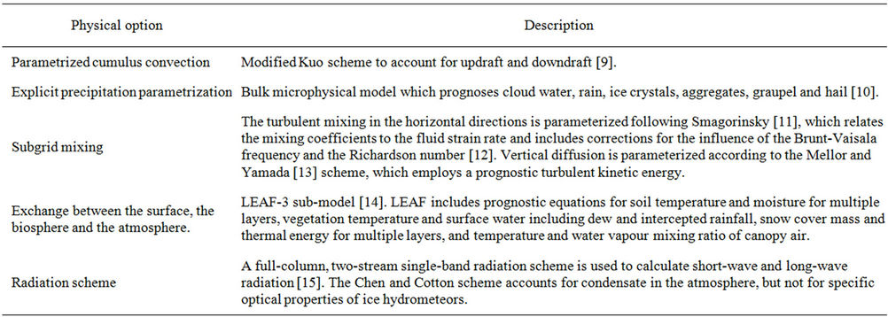
Table 2. RAMS model physical settings.
responds to 44 and 33 grid points in the North-South and West-East directions, respectively. Analyses are produced at the following twenty-three pressure levels: from 1000 to 800 hPa every 23 hPa, and form 800 hPa to 100 hPa every 50 hPa.
To show more robust statistics, and considering the data availability, analyses were computed every six hours starting from 06 UTC on 1 August and ending at 00 UTC on 11 August (41 analyses).
As stated above, the background is given by short-term forecasts of the RAMS model. In particular, two 12-h forecasts were produced daily from 1 to 10 August 2008 starting at 00 and 12 UTC. The RAMS forecast uses the ECMWF operational analysis-forecast cycle of 00 and 12 UTC as initial and dynamic boundary conditions. The 6 h and 12 hours RAMS forecasts are used as background for the analysis algorithm.
For example, referring to the 1 August, the RAMS forecast staring at 00 UTC gives the background fields for the 06 and 12 UTC analyses on 1 August, while the 12 UTC forecast gives the background fields for the 18 UTC analysis on 1 August and for the 00 UTC analysis on 2 August, and similarly for other days.
3. The Analysis System
The analysis package has different methods of solution: successive approximation, optimal interpolation and 3DVar. They are summarized in this section. The current implementation of the analysis package is univariate for all the methods.
3.1. Successive Approximation (or Correction)
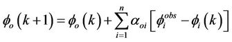
In this method two equations are iteratively solved for each analyzed variable f. The first equation is the estimate of the correction for the grid-point variable fx, the second equation is an updated observation estimate fo:
 (1)
(1)
and:
 (2)
(2)
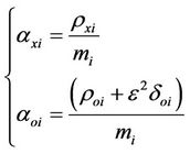
where f obsi is the value of the i-th observation, and n are the available observations. In Equations (1) and (2), k is the iteration number, and fi(k) is the first-guess estimate of the i-th observation for the k-th iteration. A few iterations are enough for the solution convergence [17], as shown in Sections 4 and 5, and in the practical implementation of the analysis algorithm, the number of iterations is set to ten. It is important to stress that the successive correction method converge to the optimal interpolation solution (see next section) as the number of iterations increases [1]. To better show how fast is the convergence of the solution, this paper shows the analysis for two (SA_2) and ten (SA_10) iterations, respectively. The grid-point analysis weight axi and the observation analysis weight aoi are given by:
 (3)
(3)
where r is the correlation function, e2 is the ratio of the observational error variance (so2) to the first-guess forecast error (sb2), which is a function of the analyzed variable and level, and doi is the Kronecker delta function.
The correlation r is a Gaussian function of the distance r. In particular:

where the length-scale d defines the observation radius of influence.
The mi is the data density and is computed as:

The aim of this paper is to show the characteristics and performance of the analysis system more than to show its benefits in the operational context and, for this purpose, its setting is compatible with real cases but not statistically optimized for the particular background used3. So, the length scale d is assumed to be 300 km for all variables at all levels. For real cases, and for optimizing the analysis solution, the length-scale can be computed for a particular background setting by the NMC method [6].
The observational error (so2) is taken from Sashegyi et al. (see Table 1 of [17]). The background error (so2) is assumed equal to the observational error. However, as shown by the application of the package, the analysis is sensitive to the value of e and its value need to be carefully estimated in future research. The method of Lönnberg and Hollingsworth ([7]) can be used for this purpose.
3.2. Optimal Interpolation
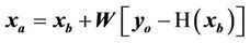
The analysed field at each vertical level is given by the equation:
 (4)
(4)
where xa is the analyzed vector, xb is the background (or first guess) field, yo is the observational vector, H is the forward observational operator, which converts the background field into first guesses of the observations, and W is the optimal weight (or gain) matrix.
The gain matrix W is given by:
 (5)
(5)
where B and R are the background and observational error covariance matrices, respectively, and HT is the transpose of the Jacobian of the forward observation operator (which transforms observation points back to grid points).
The H matrix is a bilinear interpolation operator.
The R and B matrices depend on the observation (so2) and background (sb2) error covariances, respectively, whose magnitudes were introduced in Section 3.1.
Once observation and background error covariances are determined, the matrices R and B are easily formed for each parameter. R is a p × p diagonal matrix whose elements are all equal to so2 and p is the number of observations available at the analysis time for the particular level analyzed (form 0 to 20 depending on the case). For the background error, a Gaussian shape is assumed with the (horizontal) length-scale of 300 km. So, B is an n × n matrix, where n is the number of grid-points in the horizontal analysis domain (i.e. n = 44 × 33 = 1452), whose element ij is the value of the Gaussian evaluated for the distance between the grid points i and j and multiplied by sb2.
In future implementations, the OI solution will be changed in 2D-Var, because the latter is more efficient from a computational point of view.
3.3. 3D-Var
The basic goal of the 3D-Var algorithm is to produce an optimal estimate of the true atmospheric state at analysis time through iterative solution of a prescribed cost-function ([18]):
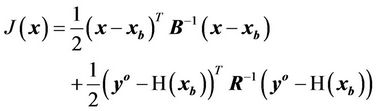 (6)
(6)
where J(x) is the costfunction, xb is the background state, H is the forward observational operator, yo is the vector of the observations, B, and R are the background, and observational error covariance matrices, respectively.
The problem can be summarized as the iterative solution of Equation (6) to find the analysis state x that minimizes J(x). This solution represents the a posteriori maximum likelihood (minimum variance) estimate of the true state of the atmosphere given the two sources of a priori data: the background xb and observations yo ([19]).
For a model state x with n degrees of freedom, calculation of the background term of the cost function requires ~ O(n2) calculations. For a typical NWP model with n ~ 105 - 107 (number of grid-points times number of independent variables) direct solution is prohibitively expensive.
One practical solution to this problem is to perform a preconditioning via a control variable v transform defined by x’ = Uv, where x’ = x – xb. The transform U is chosen to approximately satisfy the relationship B = UUT. Using the incremental formulation [20] and the control variable transform, Equation (6) may be rewritten:
 (7)
(7)
where yo’ = yo – H(xb) is the innovation vector and H is the linearization of the potentially nonlinear observation operator H used in the calculation of yo’. In this form, the background term is essentially diagonalized, reducing the number of calculations required from O(n2) to O(n). In addition, the background error covariance matrix equals the identity matrix I in control variable space, hence preconditioning the minimization procedure.
Another goal of the control variable transform is to represent spatial correlations in an accurate and simple form [21].
In the implementation of the 3D-Var scheme of this paper, the transformation U is represented by a horizontal and a vertical transformation U = UhUv. The vertical transformation has a Gaussian shape whose vertical lengthscale is constant for all variables and vertical levels. Again, the Parrish and Derber ([6]) method can be used to estimate its value to minimize the analysis RMSE for a particular background setting. In the following, the solutions using 500 m (hereafter also 3D-Var_500) and 750 m (3D-Var_750) as vertical length-scales will be shown.
The horizontal transformation Uh is given by:

where E and L are defined by:

The Bh is the horizontal component of the background error matrix and has a Gaussian shape whose length scale is 300 km. Bh is an n × n (n = 44 × 33 = 1452) matrix whose element ij is the value of the Gaussian for the distance between the grid points i and j multiplied by sb2. The background sb2 and observational sb2 errors were introduced in Section 3.1.
Theobservational error covariance matrix R is a p × p diagonal matrix whose elements are all equal to sb2 and p is the number of observations available at the analysis time for all levels.
It should be mentioned that computational issues limit the horizontal and vertical resolution using the 3D-Var approach.
It is noticed that this is the basic reason for using the successive approximation and OI methods, which are computationally less expensive than 3D-Var but twodimensional, even to solve three dimensional problems, as shown in this paper. Beside the physical nature of the problem (there are problems that are physically two-dimensional, as for example the analysis of surface parameters), when the vertical decorrelation length scale of the error is small compared to the vertical resolution of the analyses, the 3D-Var, OI and successive approximation solutions converge. For these cases, OI and successive approximations may be used to replace 3D-Var, in order to reduce the computational cost and to increase the horizontal resolution of the analyses. This point will be further discussed in Section 5.
4. Analysis Performance and Statistics
In this paragraph an example of analysis is firstly discussed to better show how the analysis system works; then statistics of the comparison between analysis and observations, and of the comparison between the background and observations are discussed.
Figure 2 shows the background, the analysis, and their difference for the temperature at 700 hPa at 00 UTC on 7 August. The analysis is produced by the 3D-Var solution with 300 km and 500 m of horizontal and vertical lengthscales, respectively. This parameter and time were selected because the difference between the analysis and background fields shows a pattern well representative of others parameters, times, and analysis levels.
The background and analysis differences are mainly concentrated over the eastern part of the domain and show a rather complex pattern. This is caused by the sign of the innovation (i.e. of the difference between the observation and the background interpolated at the observation point), which is negative for three observations and positive for the others, by the absolute value of the innovation, and by the horizontal and vertical length-scales.
Despite the differences between analysis and background fields are less than 1 K over the domain, they are well evident looking at 271 K contour near the Gotland Island, in the Baltic Sea.
Finally, it is also interesting to note the difference between the background and analysis in northern France (near Paris), which shows the effect of an insulated measurement on the analyzed field.
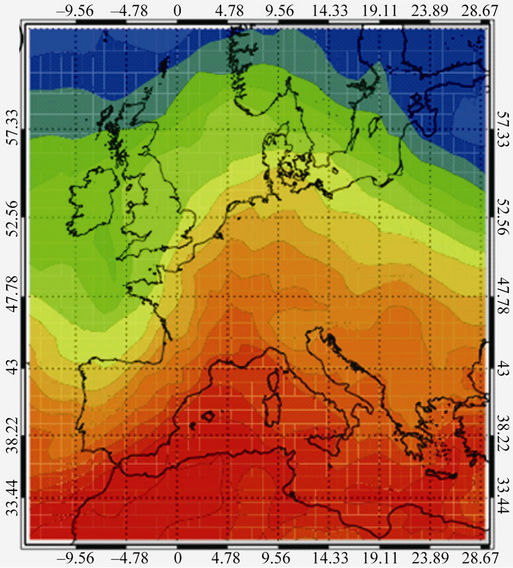
Figure 3(a) shows the RMSE between the different solutions of the analyses and observations, and the RMSE between the background and observations for the temperature.
The RMSE is computed for the whole analyses considering the grid-points of the analysis grid (Figure 1) nearest to the observations.
The background error varies between 0.8 and 1.7 K depending on the level. The analyses RMSE profiles are similar to the background but the RMSE values are almost halved. This result is expected because the observational (so2) and background (sb2) errors are equal. This means that, for an ideal case of one measurement available at one grid point of the analysis grid, the analysis at this point equally weights the observation and the background. Because only grid points nearest to the observations are used to compute the RMSE of Figure 3(a) it should be expected an almost halved RMSE for the analyses compared to the background.
Comparing the analyses RMSE it is noteworthy that:
1) The OI and SA_10 RMSE have almost the same values. As will be shown in the next section this is caused by the fact that the two analyses are almost identical.
2) As expected, SA_2 has a RMSE closer to the background compared to SA_10. However, the RMSE difference is small (0 - 0.1 K).
3) 3D-Var_750 shows a larger RMSE compared to OI below 800 hPa (RMSE 0.1 - 0.4 K larger than OI), and the smallest value between 650 and 300 hPa. Above 300 hPa the 3D-Var_750 and OI solutions have the same RMSE; as will be shown in the next section this is caused by the fact that OI and 3D-Var_750 are almost identical above this level.
4) 3D-Var_500 has an RMSE larger than OI (RMSE 0.1 - 0.2 K larger) up to 925 hPa. Above this level, its RMSE is smaller. The OI and 3D-Var_500 RMSE are almost identical above 400 hPa. Again, this is caused by
 (a)
(a) (b)
(b) (c)
(c)
Figure 2. (a) Temperature (K) background at 00 UTC on 07 August 2008 at 700 hPa; (b) Temperature analysis (K) at the same time and level of (a); (c) Difference between (b) and (a). The shaded contours are equal for (a) and (b).
the fact that OI and 3D-Var_500 are almost identical above this level.
Figure 3(b) shows the RMSE for the analyses and background for relative humidity. The background RMSE varies between 12% and 30% and increases with height. Analyses profiles follow the background behaviour but show a RMSE almost halved. Among analyses, the 3DVar_750 has the largest RMSE below 800 hPa and the lowest error above 500 hPa, while 3D-Var_500 has the smallest RMSE between 850 and 700 hPa. The SA_2 RMSE is closer to that of the background compared to SA_10, but differences are small (<2%).
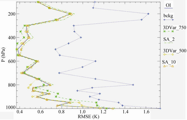
Figure 3(c) shows the RMSE for the analyses and background for the geopotential height. The background RMSE varies between 10 and 22 m with two maxima at the top and bottom of the vertical domain. The analyses have a smaller RMSE and again, the RMSE comparison shows the ability of 3D-Var to potentially reduce the error respect to two-dimensional methods (OI and successive approximation), because its solution may be sizeably different from two-dimensional methods. It should be highlighted that a lower (larger) RMSE of the 3D-Var solution does not imply a better (worse) performance of the method, unless its parameters have been determined optimally. In fact the measurements, assumed here as the reference, are not the truth. Nevertheless, the fact that 3D-Var and two-dimensional solutions are different shows that 3D-Var can improve the analysis compared to twodimensional methods, once its parameters are set optimally. The 3D-Var_500 RMSEis lower than two-dimensional methods up to 400 hPa, while its RMSE converges to OI solution above this level. Again, this is due to the convergence of the two analyses above that layer. The 3D-Var_750 analysis has the smallest RMSE above 750 hPa and the largest RMSE below 825 hPa.
Figure 3(d) shows the RMSE for the analyses and background for the zonal wind velocity. The RMSE varies between 5 m/s and 2 m/s for the background and has a maximum near the surface, showing the well known difficulties of meteorological models at reproducing the wind in the Planetary Boundary Layer and Surface Layer.
For the analyses RMSE similar considerations to other meteorological parameters apply. First their RMSE is almost halved compared to the background. In general, the 3D-Var_500 and 3D-Var_750have a lower RMSE compared to two-dimensional methods but they have a larger RMSE for lower levels, particularly the 3D-Var_750. The SA_2 shows a larger RMSE than SA, closer to the background, but the differences with SA_10 are small (<0.1 m/s). Finally, the SA_10 RMSE is very similar to that of OI. As will be shown in the next section, this is caused by the fact that OI and SA_10 analyses are very similar at all levels.
Figure 3(e) shows the RMSE for the background and analyses for the meridional wind component. The background RMSE varies between 5 m/s and 1.8 m/s. The
 (a)
(a) (b)
(b)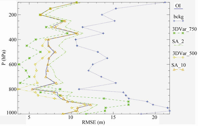 (c)
(c)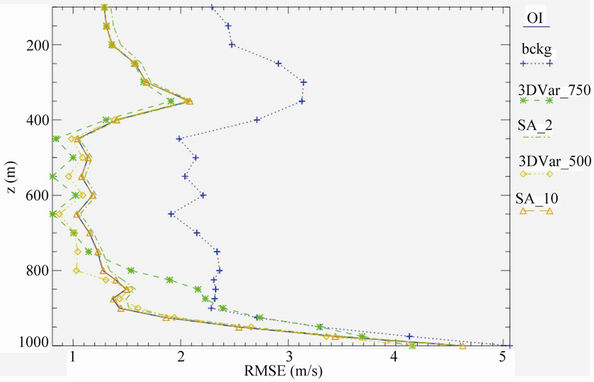 (d)
(d)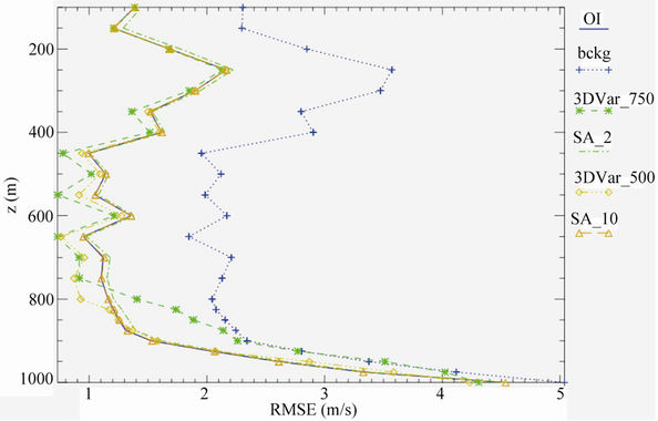 (e)
(e)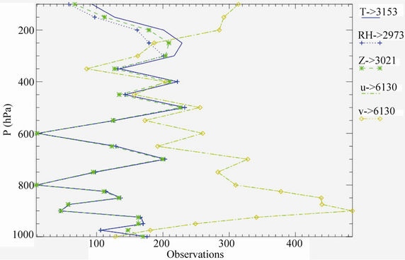 (f)
(f)
Figure 3. (a) Vertical distribution of the RMSE computed between the analyses and observations for air temperature and for different methods of solution. The background is shown for comparison; (b) As in (a) for the relative humidity; (c) As in (a) for the geopotential height; (d) As in (a) for the zonal velocity; (e) As in (a) for the meridional velocity; (f) Total number of measurements available for the analyzed parameters as a function of the level. The values shown in the legend on the right are the sum for all the levels (i.e. the total number of observations used for each parameter).
RMSE is larger in the Surface Layer and in the Planetary Boundary Layer. The analyses RMSE follow the background behaviour but their values are almost halved. For the comparison between analyses, similar considerations to other meteorological parameters apply.
Figure 3(f) shows the observations available for the analyses for each level and parameter. The average number of observations available at each level for each time is the ratio between the value of Figure 3(f) and the total analysis number (41). The larger values for the zonal and meridional wind components are caused by the use of the European wind profiler network, which reports wind components only.
5. Comparison between Methods of Solution
In this section the different methods of solution (successive approximation, optimal interpolation, and 3D-Var) are compared. The successive approximation with two and ten iterations, and 3D-Var with 500 and 750 m of vertical length-scale are considered. As discussed in Section 3, for all solutions the horizontal length-scale is 300 km, and the observational and background errors are equal.
Optimal interpolation is assumed as reference to better show the differences between the successive approximation with two and ten iterations. Again, errors are estimated for the whole dataset (41 analyses) considering only the grid-points nearest to the observations.
Only results for temperature (thermodynamic variable) and zonal wind component (dynamical variable) are shown, because similar considerations apply to other parameters.
Figure 4(a) shows the temperature RMSE. For levels below 300 hPa, 3D-Var_750 shows the largest difference compared to OI (maximum of about 1.2 K at 975 hPa), then follows 3D-Var_500 (maximum of about 1.0 K at 975 hPa), SA_2 (maximum less then 0.2 K at upper levels, namely 250 hPa), and SA_10, which shows a RMSE less then 0.1 K at all levels.
Up to 300 hPa, however, the 3D-Var solution converges towards OI both for both 500 and 750 m vertical length-scale. This is expected because at higher levels the vertical distance between analysis levels increases and becomes larger than the vertical length-scale, which quantify the vertical distance of the error decorrelation and the coupling between levels in the 3D-Var solution. As a consequence, the vertical coupling between layers becomes smaller with height, and the 3D-Var solution formally converges to OI [1].
At lower levels, where the vertical spacing between analysis levels is comparatively lower, the difference between 3D-Var and two-dimensional methods becomes larger.
This point is of practical importance because it shows that two-dimensional methods can be used when the vertical error decorrelation length-scale is smallcompared to the vertical spacing of the analysis grid (as for upper levels). For example, the two-dimensional methods of this paper can be used in synergy with 3D-Var by dividing the three-dimensional domain in two subdomains: an upper part and a lower part. The two dimensional methods can be used for the upper part and the 3D-Var can be used for the lower part, without losing accuracy of the analyzed field but decreasing the number of grid-points in each subdomain. This decomposition can be used for reducing the computational resources and/or for increasing the horizontal resolution of each subdomain.
Figure 4(a), as expected, shows thatthe successive approximation with ten iterations is closer to OI compared to the same solution with two iterations at all levels, but it is worth noting that the convergence of the successive approximation scheme is fast because the RMSE between SA_2 and OI is less than 0.1 K at all levels, which is a small value from a practical point of view. This result is important, because only few iterations need to be performed when using the SA scheme.
Figure 4(b) shows the zonal wind component RMSE. In general, similar considerations of Figure 4(a) apply. The 3D-Var solution with 750 m vertical length-scale shows the largest differences (up to 3.6 m/s at 950 hPa) respect to OI; then follows 3D-Var with 500 m of vertical length-scale (2.6 m/s of maximum RMSE at 975 hPa).
As expected, the successive approximation with ten iterations is closer to OI compared to the same solution with two iterations and its RMSE is lower than 0.2 m/s for all levels.
6. Conclusions
This paper shows the performanceof a general purposes analysis package able to solve twoand three-dimensional problems adopting the following solutions: successive approximation, optimal interpolation, and 3D-Var. The package is able to ingest the data from the following observations of the GTS network: synop (non considered in this paper), TEMP, and wind profilers. It performs the analysis of the following parameters: zonal and meridional wind components, temperature, geopotential height, relative humidity, and surface parameter (not considered in this paper).
Main conclusions may be summarized as follows:
1) All the analyses solutions perform well; for the particular setting of the analysis package, and for the verifying method used, it is expected that the analyses RMSEs, computed assuming the observations as the reference, are almost halved compared to the background RMSE. This
 (a)
(a)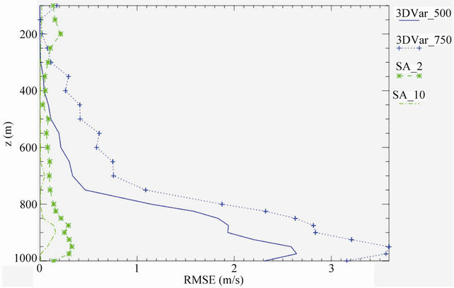 (b)
(b)
Figure 4. (a) RMSE between Optimal Interpolation and other solution methods for temperature; (b) As in (a) for the zonal wind component.
was verified for all solutions.
2) The successive approximation scheme quickly converges to the OI solution. It was shown that even if the SA_10 is closer to OI than SA_2, the differences between SA_2 and OI are small in absolute values for all parameters, at least for the setting adopted in this paper.
3) The 3D-Var solution converges to OI when the error vertical decorrelation length-scale become small compared to the vertical spacing of the analysis grid.
4) The 3D-Var solution shows the potential to produce analyses with a lower RMSE (computed respect to the truth) compared to two-dimensional methods.
5) The results of this work highlight the importance of optimally determining the parameters of the analysis method, namely the horizontal and vertical length-scales and the observational and background errors, trough statistical methods as shown in [6,7].
Finally, it is remarked that work is in progress to implement a 2D-Var solution, which is computationally more efficient than OI, and to test the analysis package in a real forecast context.
7. Acknowledgments
This paper was realized within the APQ Az. 3 Filiera vitivinicola-MAPVIC project, funded by the Calabria Region. The author is grateful to the ECMWF for both the support and for the access to the MARS database.
REFERENCES
- E. Kalnay, “Atmospheric Modeling, Data Assimilation and Predictability,” Cambridge University Press, Cambridge, 2003.
- D. M. Barker, Huang, W., Y. R. Guo and Q. N. Xiao, “A Three-Dimensional Variational Data Assimilation System For MM5: Implementation and Initial Results,” Monthly Weather Review, Vol. 132, No. 4, 2003, pp. 897-914. doi:10.1175/1520-0493(2004)132<0897:ATVDAS>2.0.CO;2
- S. M. Lazarus, C. M. Ciliberti, J. D. Horel and K. A. Brewster, “Near-Real-Time Applications of a Mesoscale Analysis System to Complex Terrain,” Weather and Forecasting, Vol. 17, No.5, 2002, pp. 971-1000. doi:10.1175/1520-0434(2002)017<0971:NRTAOA>2.0.CO;2
- F. Zhang, Z. Meng and A. Askoy, “Tests of an Ensemble Kalman Filter for Mesoscale and Regional-Scale Data Assimilation. Part I: Perfect Model Experiments,” Monthly Weather Review, Vol. 134, No. 2, 2006, pp. 722-736.
- A. D. Schenkman, M. Xue, A. Shapiro, K. Brewster and J. Gao, “The Analysis and Prediction of the 8-9 May 2007 Oklahoma Tornadic Mesoscale Convective System by Assimilating WSR-88D and CASA Radar Data Using 3DVAR,” Monthly Weather Review, Vol. 139, No. 1, 2011, pp. 224-246. doi:10.1175/2010MWR3336.1
- D. F. Parrish and J. C. Derber, “The National Meteorological Center’s Spectral Statistical Interpolation Analysis system,” Monthly Weather Review, Vol. 120, No. 8, 1992, pp. 1747-1763. doi:10.1175/1520-0493(1992)120<1747:TNMCSS>2.0.CO;2
- P. Lönnberg and A. Hollingsworth, “The Statistical Structure of Short-Range Forecast Errors as Determined from Radiosonde Data. Part II: The Covariance of Height and Wind Errors,” Tellus, Vol. 38A, No. 2, 1986, pp. 137-161. doi:10.1111/j.1600-0870.1986.tb00461.x
- W. R. Cotton, R. A. Pielke Sr., R. L. Walko, G. E. Liston, C. Tremback, H. Jiang, R. L. McAnelly, J. Y. Harrington, M. E. Nicholls, G. G. Carrio and J. P. McFadden, “RAMS 2001: Current Satus and Future Directions,” Meteorological and Atmospheric Physics, Vol. 82, No. 1-4, 2003, pp. 5-29. doi:10.1007/s00703-001-0584-9
- J. Molinari and T. Corsetti, “Incorporation of Cloud-Scale and Mesoscale Down-Drafts into a Cumulus Parametrization: Results of One and Three-Dimensional Integrations,” Monthly Weather Review, Vol. 113, No. 4, 1985, pp. 485- 501. doi:10.1175/1520-0493(1985)113<0485:IOCSAM>2.0.CO;2
- R. L. Walko, W. R. Cotton, M. P. Meyers and J. Y. Harrington, “New RAMS Cloud Microphysics Parame-terization. Part I: The Single-Moment Scheme,” Atmospheric Research, Vol. 38, No. 1-4, 1995, pp. 29-62. doi:10.1016/0169-8095(94)00087-T
- J. Smagorinsky, “General Circulation Experiments with the Primitive Equations. Part I: The Basic Experiment,” Monthly Weather Review, Vol. 91, No. 3, 1963, pp. 99-164. doi:10.1175/1520-0493(1963)091<0099:GCEWTP>2.3.CO;2
- R. A. Pielke Sr., “Mesoscale Meteorological Modeling,” Academic Press, San Diego, 2002.
- G. Mellor and T. Yamada, “Development of a Turbulence Closure Model for Geophysical Fluid Problems,” Reviews of Geophysics and Space Physics, Vol. 20, No. 4, 1982, pp. 851-875. doi:10.1029/RG020i004p00851
- R. L. Walko, L. E. Band, J. Baron, T. G. Kittel, R. Lammers, T. J. Lee,D. Ojima, R. A. Sr. Pielke, C. Taylor, C. Tague, C. J. Tremback and P. L. Vidale, “Coupled Atmosphere-Biosphere-Hydrology Models for Environmental Prediction,” Journal of Applied Meteorology, Vol. 39, No. 6, 2000, pp. 931-944.
- C. Chen and W. R. Cotton, “A One-Dimensional Simulation of the Stratocumulus-Capped Mixed Layer,” The Boundary Layer Meteorology, Vol. 25, 1983, pp. 289-321. doi:10.1007/BF00119541
- S. Federico, “Verification of Surface Minimum, Mean, and Maximum Temperature Forecasts in Calabria for Summer 2008,” Natural Hazards and Earth System Sciences, Vol. 11, No. 2, 2011, pp. 487-500. doi:10.5194/nhess-11-487-2011
- D. K. Sashegyi, D. E. Harms, R. V. Madala and S. Raman, “Application of the Bratseth Scheme for the Analysis of GALE, Data Using a Mesoscale Model,” Monthly Weather Review, Vol. 121, No. 8, 1993, pp. 207-220. doi:10.1175/1520-0493(1993)121<0207:AOVMIT>2.0.CO;2
- K. Ide, P. Courtier, M. Ghil and A. C. Lorenc, “Unified Notation for Data Assimilation: Operational, Sequential and Variational,” Journal of the Meteorological Society of Japan, Vol. 75, No. 1B, 2011, pp. 181-189.
- A. C. Lorenc, “Analysis Methods for Numerical Weather Prediction”, Quarterly Journal of the Royal Meteorological Society, Vol. 112, No. 474, 1982, pp. 1177-1194. doi:10.1002/qj.49711247414
- P. Courtier, J. N. Thépaut and A. Hollingsworth, “A Strategy for Operational Implementation of 4D-Var, Using an Incremental Approach,” Quarterly Journal of the Royal Meteorological Society, Vol. 120, No. 519, 1994, pp. 1367-1387. doi:10.1002/qj.49712051912
- D. M. Barker, W. Huang, Y-R. Guo, A. J. Bourgeois and Q. N. Xiao, “A Three-Dimensional Variational Data Assimilation System for MM5: Implementation and Initial Results,” Monthly Weather Review, Vol. 132, No. 4, pp. 897-914. doi:10.1175/1520-0493(2004)132<0897:ATVDAS>2.0.CO;2
NOTES
1The analyses can also be produced for surface meteorological parameters (not shown in this paper), namely: temperature, relative humidity, and wind.
2This point can be of practical importance in the operational implementation of the analysis scheme.
3To optimize the method statistically, the observational and background errors and the horizontal (and vertical in the case of 3D-Var) lengthscale must be selected to minimize the RMSE between the analyses and the unknown truth. The references [6], [7], and [1] discusses how to optimize the analyses.