Atmospheric and Climate Sciences
Vol. 2 No. 1 (2012) , Article ID: 17129 , 13 pages DOI:10.4236/acs.2012.21009
Distinct Global Patterns of Strong Positive and Negative Shifts of Seasons over the Last 6 Decades
1Department of Forest Ecosystems and Society, Oregon State University, Richardson Hall, Corvallis, USA
2Institute of Landscape Ecology, Department of Climatology, University of Münster, Münster, Germany
Email: *andres.schmidt@oregonstate.edu
Received October 29, 2011; revised December 5, 2011; accepted December 23, 2011
Keywords: Climate Change; Temperature Phase Shift; Neural Networks; Phenology; Near-Surface Temperature
ABSTRACT
Alterations of annual temperature cycles have profound implications on how the planet responds to global climate change. In this study, a high resolution global analysis of temperature cycle shifts and their development over time is presented. We show that over the last 63 years, phase shifts in the annual near surface temperature cycle exhibit large spatiotemporal variability. The calculated phase shifts comprise earlier onsets of seasons as well as delays with similar frequencies, depending on location. From 1978 to 2010 Eastern Europe experienced an advanced annual cycle of near-surface temperature of 3.2 days while Eastern Australia shows an opposite shift towards later seasons of 3.5 days in comparison to the preceding 30-year period from 1948 to 1977. The largest phase shifts of –5.5 days toward earlier seasons over land were found in Belarus and Northwest Russia. For the first time the developments of seasonal temperature shifts were generalized for large areas by using self-organizing feature map neural networks resulting into 4 significant global trends. The temperature phase shifts are also shown to have strong correlations with the timing of shrub foliation observed at 57 phenological stations across the USA. The findings have far-reaching, yet regionally distinct consequences on agriculture, animal life cycles, plant phenology, and regional weather phenomena that change with annual temperature cycles.
1. Introduction
Climate change is associated with momentous consequences on vital aspects of human life. Acting through diverse and complex interdependencies, greenhouse gas driven warming is predicted to have large impacts on agriculture, the frequency and intensity of droughts and extreme precipitation events, drinking water supply, species migration and conflicts over resources [1]. While an increasing atmospheric CO2 concentration causes the average global temperature to rise, the complex manner in which the climate system transports energy causes long-term trends of temperature to differ by region and season. The strongest warming within the last century was found in continental areas of the middle and higher latitudes especially a warming of the winter periods. Other regions, including parts of the northern Atlantic, the southern oceans, and parts of Antarctica actually cooled [1-5]. In addition to warming, or changes in the temperature amplitude, changes in the phase of annual cycle of air temperature have been shown in analyses of several datasets using a variety of methods [6-11].
Stine et al. [10] found that the temperature cycle advanced by 1.7 days between 1954 and 2007 over extra-tropical land, based on an averaged yearly shifts between monthly values of local solar insolation and surface temperature. Thomson [6] discovered a coherency between the average change in phase and the logarithm of atmospheric CO2 concentration for Central England. Both studies, however, were affected by significantly large data gaps. Also correlations between large-scale atmospheric circulation systems and the earlier onset of spring were found in several studies [9,12-14] indicating the complex interdependencies between changes in the large-scale climate system and the phase of the annual temperature cycle and associated seasons. Nevertheless, the understanding of seasonal shifts and spatial patterns of global temperature trends over time, however, has been restricted by limitations in observations and associated scaling. Mechanisms by which warming through increasing atmospheric CO2 concentrations may cause shifts in the timing, duration, and intensity of the annual temperature cycle are not captured by current global models [10].
Several recent phenological studies also show an earlier onset of spring and describe strong associations of this pattern with changes in the temperature cycle [15- 18]. Parmesan [19] analyzed the phenological response of 203 different species on the northern hemisphere including plants, birds, butterflies, and fish and found significant differences in the strength of response to the changed annual temperature cycles across geographic and taxonomic groups.
Changes in the timing of the annual temperature cycle and the related altered onset of spring have also been shown to impact the amount of CO2 exchange, greenness index [18] and albedo of vegetated regions. Also an increased frequency of wildfires is associated with corresponding earlier onsets of spring in Western USA [20].
These examples underline the importance of the phase shift and its effects on complex interactions between the phase of the temperature and dependent processes in our environment, while the extensive and complex reactions of ecosystems to changes in the seasonal cycle are still far from being understood or predictable.
Hence, beyond proven effects on lifecycles of plants and animals [15,16,19], these phase shifts are an indicator for ongoing momentous changes in the climate system whether they are directly related to the global warming trend or not.
It is important to note that an earlier onset of spring associated with a threshold temperature reached earlier in the year should not be confused with the phase shift of the annual cycle. A general increase of mean annual temperature consequently leads to an extended growing season and an earlier start of spring. A phase shift, however, can be negative or positive. Hence, in contrast to this effect of a generally higher mean annual temperature, a phase shift could lead to an advanced or delayed start of the growing season. In fact, the known changes of annual temperature amplitudes are superimposed by phase shifts of the air temperature time series [10,11].
In this study we focus on the phase shifts between temperature series of different periods using a crossspectrum analysis approach [21,22] and a combination of a self-organizing feature map (SOFM) neural network [23,24] and a subsequent k-means clustering. The used NCEP/NCAR Reanalysis 1 temperature dataset with a 2.5˚ resolution covers the last six decades and is spatially comprehensive. This high resolution enables us to also assess the phase shift over vast areas on the southern hemisphere and apply a pattern recognition algorithm on the global distribution of the phase shifts of the annual temperature cycle for the first time.
2. Data and Methods
2.1. The Reanalysis Dataset
By comparing two continuous segments of one distinct temperature time series for each point of a global grid a statistically significant calculation of the long-term shift of the annual temperature cycle was achieved. For this purpose, the time series were divided into two 30-year segments. According to WMO standard, only periods of 30 years or more are considered long enough to safely account for the effects of natural short-term variations and are therefore suitable for analyses of long-term climate effects [25,26]. The first fraction of the used series covers the period 1948 through 1977. This was considered the 30-year early reference period. The second part of the spatially apportioned series is from 1981 through 2010. Thus, both 30-year periods are separated by a three-year gap with the data of 1978 to 1980. One effect of the three year gap is that the two sequences of the time series can be considered clearly independent from each other in terms of the persistence interval inherent to air temperature series. Secondly this separation was made according to the anomalies of the global near surface air temperature [3,5,27]. The early 1980s to 2010 are characterized by an increase of positive temperature anomalies as compared to previous decades and were chosen as the second period (Figure 1).
For the cross-spectrum analyses applied to the detrended data series of each grid point we used the global NCEP/NCAR Reanalysis 1 dataset with a 2.5˚ × 2.5˚ resolution provided by the NOAA/OAR/ESRL PSD, Boulder, Colorado, USA [29,30]. For the benefit of the explanatory power of derived phase shift values and trends the dataset exhibits no gaps and provides a globally complete spatial coverage.
We extracted a global dataset consisting of 10,512 time series for each grid point, containing the daily near surface air temperature values from the beginning of 1948 to the end of 2010. Due to the Nyquist frequency restrictions, a second corresponding dataset with a 6-hourly temporal resolution was used to safely exclude time series whose biggest part of the spectral variance was not caused by
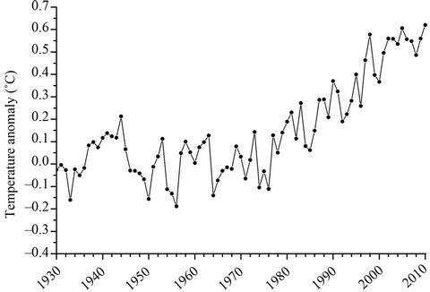
Figure 1. The annual anomalies of the global surface air temperature based on the 20th century average [28].
the annual (i.e. seasonal) cycle but was associated with lower or higher frequencies. This excluded a vast part of the tropical regions where the diel variance in temperature is much higher than the variance on the annual time scale. The 1000 hPa temperature series used in this study exhibit the highest available data quality level A because the respective modeled values are highly influenced and evaluated by measured temperature values [29]. It should be noted that the availability of meteorological reference measurements available for the Arctic and Antarctica was limited. Nevertheless, the reliability of the widely used NCEP/NCAR Reanalysis 1 temperature dataset has been discussed and proven in numerous studies [29,31, 32].
2.2. The Cross-Spectrum Analyses
As a consequence of the applied cross-spectrum method, the global shifts of the annual temperature cycles presented are not adulterated by superimposed changes of the amplitudes of the temperature series over time caused by long-term temperature trends such as global warming.
In fact, the accuracy of the calculated phase shifts only depends on the precision of the relative course of the temperature rather than being affected by uncertainties of the absolute temperature values.
The Fourier cross spectrum function P over all harmonics h of the periodic temperature time series can be separated into its real and imaginary part, i.e. in its cospectrum Co and quadrature spectrum Qu, respectively (Equation (1)).
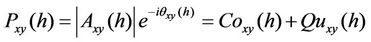 (1)
(1)
The phase shift value θxy between the time series can then be calculated with the phase spectrum function  given through,
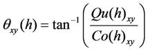 (2)
(2)
and then transformed from radians into a time value t by using
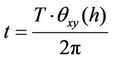 (3)
(3)
Here, T is the period of one cycle, in our case one year.
2.3. Finding Regional Trends in Phase Shift Using SOFM Networks
To find general global trends in the phase shifts between the earliest reference period (1948-1957) and the following decades we calculated 53 consecutive shifts of the annual temperature cycle for each grid point using a moving-window analysis with one-year steps and a tenyear window width. The 10-year window was chosen to accunt for year-to-year variability.
In order to cluster the resulting, spatially assigned sliding-window dataset, a SOFM neural network using Gaussian distance functions was used. SOFM networks have been successfully used to find patterns in high-dimensional and large datasets [33-36].
A first SOFM network was applied to detect outliers in the 53-dimensional temporal patterns of the one-year steps and a ten-year window phase shifts.
The network consisted of 144 neurons hexagonally arranged as a 12 × 12 lattice. The application of a hexagonal layout provides a better topology preservation of the input data compared to other feature map layouts [37]. Radial basis functions were used to calculate the neighbourhood activation values. The distances between the organized neurons at the end of the adoption procedure were determined.
Since the number of neighbours for each neuron varies within the net grid, the distances of each neuron to all of its neighbour neurons was averaged instead of comparing just the sum of the neighbour distances.
If the average of Euclidian distance considering all its neighbours Dj of a neuron is higher than 3 times the distance average calculated over all 144 neurons, a neuron was considered an outlier. The applied outlier detection rule is given by,
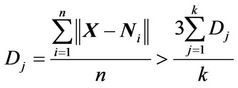 (4)
(4)
here, the position of the weight vector of the respective neuron j in the 53-dimensional input space is given by the vector X.
The vector N is the corresponding position of the weight vector of a neighbour neuron i, n gives the total number of neighbours of neuron j in the self-organizing feature map lattice, and k is the total number of neurons in the lattice.
Hence, to obtain a good generalization of the temporal phase shift patterns, the values assigned to those outlier neurons were excluded from further analyses because the associated temporal phase shift patterns are very different from all the other temporal patterns that were observed globally.
After excluding outliers as well as the vectors from areas that showed spectra with the highest variance attributed to sub-yearly temperature cycles, the remaining input data consisting of 461,312 phase shift values (8704 grid points × 53 temporal moving-window steps) was presented to a new SOFM with the same topology for the second SOFM clustering run. The resulting 144 SOFM neurons that represent the SOFM clusters after the training procedure where then merged into the 4 final clusters by using a k-means clustering algorithm. To summarize the global patterns, the best number of final clusters for the k-means procedure was determined by using the Davies-Bouldin validity Index [38-40].
3. Results and Discussion
3.1. Global Long-Term Phase Shifts
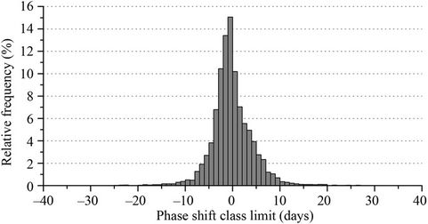
The majority (96.2%) of the local phase shifts of the annual temperature cycle between the two 30-year segments, hereafter referred to as the long-term phase shifts, occur in the range of –10 to +10 days and 81.2% are in the range of –5 to +5 days (Figure 2). This long-term phase shifts can be considered an average of the last 30 years.
Here, a positive phase shift means that the phase of the later time series (1981-2010) is delayed compared to the reference period (1948-1977), whereas a negative phase shift means that the temperature cycle of the later time series is shifted towards earlier seasons compared to the reference period. Outliers and extremely rare phase shifts that exceeded ±10 days were excluded with respect to the frequency distribution of calculated long-term shifts. Areas that exhibited maxima in the variance spectrum of their respective temperature time series that were not caused by a yearly temperature cycle but attributed to fluctuations at higher frequencies were also excluded
 (a)
(a)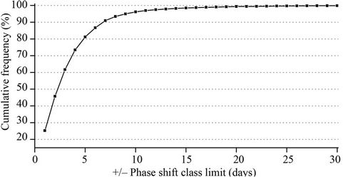 (b)
(b)
Figure 2. The relative frequency distribution (a) and the cumulative frequencies (b) of the global long-term phase shifts (1981-2010 vs 1948-1977).
from further analyses. This applied to the majority of the tropical regions.
A map with gridded results of all cross-spectrum phase shift analyses for the two 30-year periods is given in Figure 3.
A belt along the mid latitudes of the oceans of the southern hemisphere is evident, showing positive time shifts. It is interrupted by areas of South America and Australia that exhibit negative phase shifts (earlier seasons).
Within this belt between 15˚ and 55˚ South, the oceans show a positive shift, the annual temperature cycle is delayed by 4.52 days (±1.95 days standard deviation) on average in the period from 1981 through 2010 in comparison to the earlier climate period from 1948 through 1977 (Figure 3).
Many spatial agglomerations of areas that exhibit similar long-term phase shift are evident such as the major part of the Australian inland with a phase shift of –2.41 (±0.82) days, as well as Tasmania with –3.76 (±0.1) days. By contrast, Northeast Australia exhibits a shift that is associated with a time delay of the current cycle of +3.51 (±2.7) days. This result is in accordance with a long-term study at 11 wine-growing sites in Australia. The study shows an advanced maturity of wine grapes, associated with an earlier onset of spring in Southeast Australia. However, a delayed maturity of 0.1 days per year was observed at a site located in Southwest Australia [41].
The direction and magnitude of the calculated longterm shift of –1.44 days over Northeast China (Figure 3) matches the results of a long-term study in Beijing based on a local time series [11].
Over Europe, an east-west gradient is noticeable where the highest negative shifts of –3.16 (±2.03) days, associated with an earlier onset of spring, were found in Eastern and Central Europe. Globally, the highest phase shifts of –5.5 days towards earlier seasons on land were found in regions in Belarus and Northwest Russia. The temperature in Alaska shows the highest phase shifts of its annual cycle in North America with –4.9 days during the last 30 years.
Over the vast area of Russia, the annual cycle of temperature is shifted by –2.44 (±1.36) days on average, whereas the long-term shift over Western Europe including most parts of France, Spain, Portugal, Ireland, and Great Britain is considerably smaller with –0.8 (±0.37) days.
A noticeable spatial variance of the shifts in the temperature cycle was also observed across the continental USA. A west-east gradient shows a maximum negative shift of –3.04 (±1.54) on the West Coast (Washington, Oregon, and California) followed by the areas in the Midwest –2.25 (±1.28), whereas the southeast USA

Figure 3. Spatial distribution of the long-term temperature phase shifts for all grid cells with a predominant annual cycle of the near-surface air temperature.
including Florida, South Carolina, and Southeastern Alabama exhibits a positive shift of 0.78 (±0.57) days during the last 30 years on average.
The oceans also show earlier as well as later phases of the annual temperature cycle depending on their locations. A clear annual cycle of the sea surface temperature, also incorporating the tropics, has been shown in previous studies [42,43].
With the exception of the Antarctic Peninsula and adjacent waters of the Weddell Sea and Ross Sea, the Antarctic continent is also affected by an advanced yearly cycle with an average temperature shift of –1.9 (±1.46) days. The effects of large ocean currents on surface temperature lead to local temperature regimes that are reflected in the spatial patterns of temperature cycle shifts. The geographic position of these areas conforms to the position of major ocean gyres.
This can be observed in the area of North Pacific gyre that is surrounded by the mainstreams of the Alaska current and the Oyashio current. Moreover, the area that is surrounded by the North Atlantic gyre created by the Gulf Stream and the Canary current, respectively is clearly visible and centered at 40˚ North and 50˚ West.
The average phase shift values on a global and continental scale are given in Table 1.
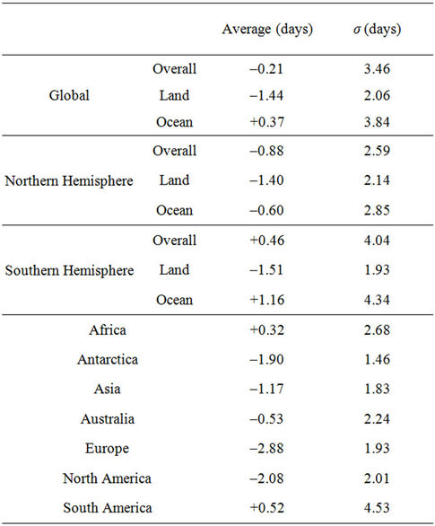
Table 1. Large-area averages and standard deviations of longterm temperature phase shifts.
This in particular affects the informative value of global and hemispheric averages. Nevertheless, with exception of Africa and South America the annual temperature cycle of the continents exhibit phase shift averages between 0.5 and almost 3 days towards earlier seasons. The spatial coverage of the continents is as given in Figure 3. Most of these large area values show high standard deviations caused by the high spatial variance evident in the results (Figure 3).
3.2. Temperature Shift Driven Changes of Phenological Events
In order to assess the effects of the temperature phase shift on phenological events and to validate the method used to calculate the phase shift values, the long-term North American First Leaf and First Bloom Lilac Phenology dataset was compared to the corresponding shifts of the temperature cycle based on the NCEP/NCAR Reanalysis 1 dataset. Starting 1956 lilac shrubs (Syringa chinensis clone and Syringa vulgaris) were planted across the USA and the dates of the first leaf were recorded annually [17,44-46]. Because the first bloom is strongly controlled by photoperiod [47] while the beginning of foliation is strongly controlled by temperature [48], the “first leaf” record was used as indicator to analyze the effect of the temperature phase shift.
The lilac “first leaf” time series have a length of 3 to 23 years with an average of 10.6 years.
A moving-window analysis (1-year steps and 1-year window width) was applied to calculate annual phase shifts from the Reanalysis 1 temperature dataset for the periods with available lilac data. Only meaningful and statistically significant correlations with a Pearson coefficient r of at least ±0.4 and p < 0.1 are shown.
The results show that 82.5% of the phenological time series exhibits a correlation coefficient of +0.6 or higher with the corresponding temperature phase shift time series for the respective area (Figure 4).
The occurrence of weak correlations (r < 0.4) or high negative correlations indicates that parameters, other than air temperature influence the life cycle of the plants and thus the day of “first leaf”. In particular, radiation and water availability are also considered to drive foliation and influence its timing [49].
The mostly high positive correlations show that changes in the phase of the temperature cycle exert strong effects on the life cycle of plants. As the foliation of trees and shrubs is directly related to their ability to assimilate carbon, the results also imply the existence of a strong effect of the phase shifts on vegetation carbon dynamics on a global scale.
Unfortunately, long term phenological records are largely confined to North America and Europe, limiting our ability to make larger scale conclusions about the phenological impacts of seasonal shifts in temperature cycles.
Nevertheless, the North American First Leaf and First Bloom Lilac Phenology dataset represents a well-documented long-term dataset that covers various climates and growing conditions in the mid-latitudes.
For the correlation analyses of the annual temperature shift values derived from the Reanalysis 1 dataset and the annual phenological shifts of the first leaf lilac dataset,
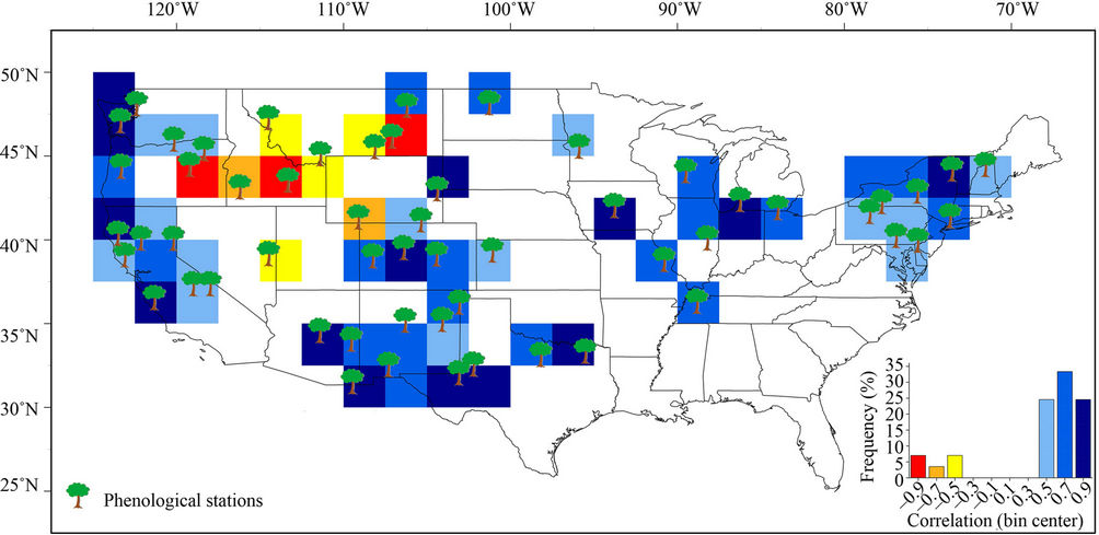
Figure 4. Correlations between the time series of the annual temperature cycle and the time series of the North American first leaf lilac phenology dataset.
the phenological sites were assigned to the closest grid point of the 2.5˚ × 2.5˚ Reanalysis 1 dataset as given in Table 2.
In cases where more than one site was close to the grid point and all of the points fulfilled the significance requirements for the correlation analysis with the temperature phase shift series, the station with the longest dataset was chosen.
All correlations are significant on a confidence level of 90% or higher. The p-values for the Pearson correlation factors r were tested using Student t significance tests.
The p-values, given in Table 2 for the two-tailed tests, were calculated conservatively by doubling the more significant of the respective two one-tailed p-values.
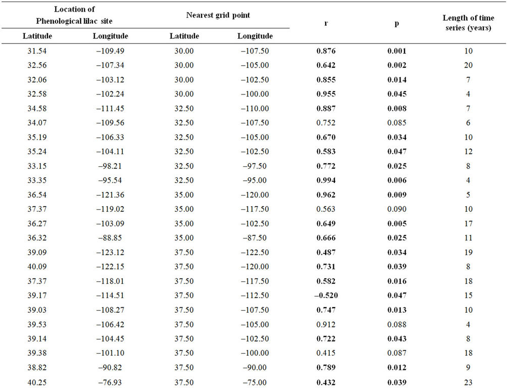
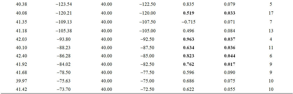
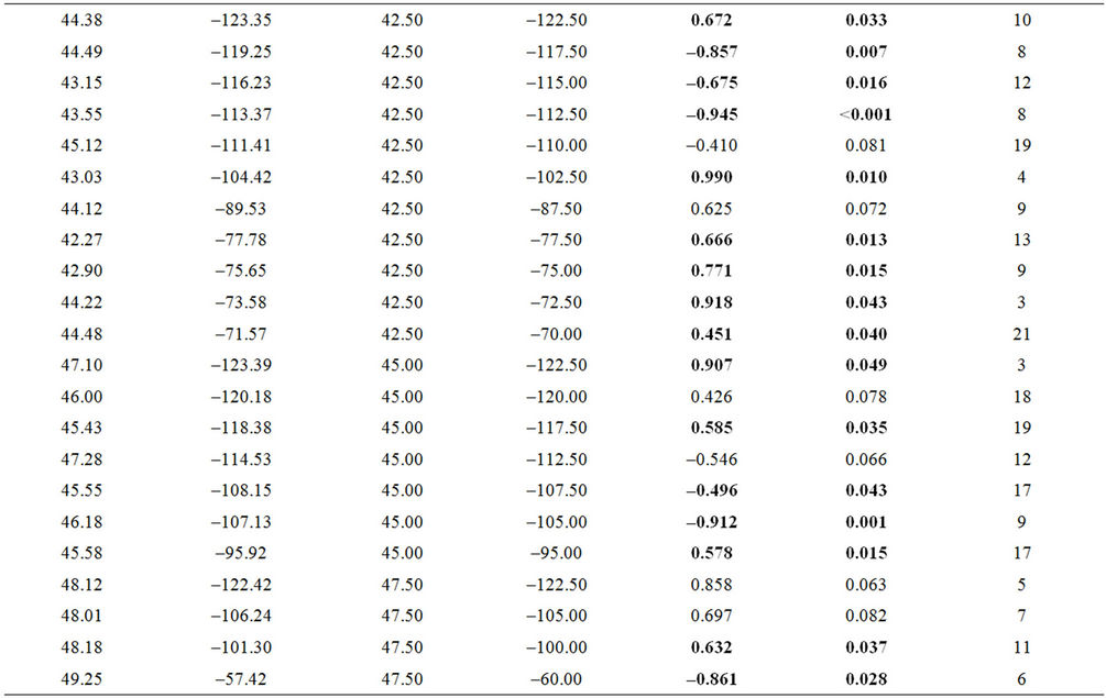
Table 2. The locations and statistical parameters for the intercomparison of shifts of the temperature cycle and associated phenological shifts. Values that are significant on a 95% level are bold.
3.3. Spatiotemporal Patterns of the Temperature Phase Shifts
To examine the development of the annual temperature phase shifts over the last six decades while accounting for spatial variances, the annual phase shift was analyzed by finding spatial similarities in the temporal patterns rather then using simple geographic subdivisions like the hemispheres or continents.
The temporal courses of the phase shifts were clustered using a SOFM neural network in connection with an ensuing k-means clustering procedure.
The Davies-Bouldin index for various numbers of trend-clusters is given in Figure 5. The input values for the SOFM network clustering were not normalized before being presented to the network as the inputs of all 53 dimensions were given in the same unit as phase shift  in days.
The Davies-Bouldin index reached a minimum when the 144 SOFM clusters were merged to 4 final clusters (Figure 5) indicating that the separation was best in terms of getting a high similarity within each cluster in combination with a high dissimilarity between the 4 clusters. This two-step clustering has been proven to provide a more accurate summarization of multidimensional input data than a single SOFM clustering or kmeans clustering approach alone. Moreover, because the
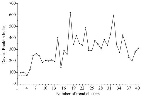
Figure 5. The cluster separation performances over 40 clusters expressed by the corresponding Davies-Bouldin validity index.
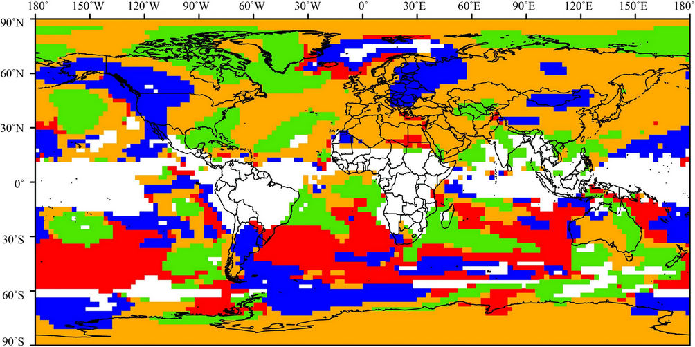
pre-clusters built by the SOFM are local averages of the raw values, the final k-means clustering is less sensitive to random variations than a direct k-means clustering of the original data [36,50]. The clustering result shows four very different temporal patterns and trends in the developments of the shifts of the yearly temperature cycles (Figures 6(a) and (b)).
Clusters 1 and 2 exhibit trends towards positive shifts whereas clusters 3 and 4 show development towards negative phase shifts (Figure 6(b)). In comparison to the
 (a)
(a)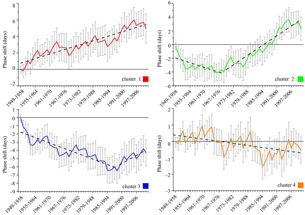 (b)
(b)
Figure 6. Spatial distribution and the courses of the clustered annual phase shifts using 10-year comparison periods. The gray error bars show the ±1σ standard deviations. The dashed lines show the linear trends (p < 0.01). Note the different scales of the vertical axes.
steep descent of cluster 3, however, the temperature shift in the areas assigned to cluster 4 shows a less pronounced trend in the first five decades of the analyzed period.
The averages of the spatially corresponding long-term shift shown in (Figure 3) also indicate that the phase of the temperature cycle during the recent 30 years is remarkably ahead of the temperature cycle during the early period from 1948 through 1977. The associated areas exhibit the strongest negative averaged long-term phase shift of –3.12 days (Table 3).
The global spatial assignments to these phase shift clusters are shown on the map in Figure 6(a). A comparison of Figures 3 and 6 shows that the assignment of areas according to their long-term shift leads to similar spatial patterns as an apportionment based on the development of the phase shifts over time. To check the statistical significance of trends of the clustered temporal courses of the phase shift, two-tailed Mann-Kendall trend tests were applied. The tests proof that all trends given in Figure 6(b) are significant on a 99% confidence level. To account for temporal changes of the course of the phase shift in the areas assigned to cluster 2 and 3, the respective linear regressions were calculated for two periods.
The distinct areas over the West Atlantic, Western China, and the Antarctic Peninsula for instance, which differ from their surrounding vicinity in terms of their long-term shift (Figure 3), are also assigned to different trend clusters than the respective neighboring areas (Figure 6(a)). In addition to short-term fluctuations, the courses of the clustered phase shift values show clear trends.
The linear trends in the areas assigned to clusters 1 and 4 are monotonically increasing or decreasing, respectively. By contrast, the linear trends of the phase shift values show a noticeable change in central and southeast Europe as well as in the Western USA (both cluster 3), beginning in the late 1980s when the trend turns from an earlier to later phase shift. Nevertheless, the phase shift shows that the temperature cycle of the most recent decade from 2001 to 2010 is still +4.2 (±1.6) days ahead of the temperature cycle during the reference decade 1948- 1957, averaged over the areas assigned to cluster 3.
The course of the phase shifts calculated for cluster 2 also exhibits a change in direction in the late 1970s (Figure 6(b)). The local phase shifts summarized in cluster 2 show an inflection point in the temporal course from negative to positive phase shifts. Here, the temperature cycle of the following years used to be ahead of the temperature cycle of the reference decade (1948-1957) until the late 1990s. Thereafter, the temperature cycle is delayed in comparison to the reference decade as a result of a relative phase shift of about 2 days.
The standard deviations given in the long-term shifts are attributed to the spatial variations within the clusters. The temporal patterns of the phase shift in combination with the maps given in Figures 3 and 6(a) show that the phase shift values are varying significantly over space and over time. This partially explains the discrepancy between the finding of Thomson [6] who used a longterm central England time series, and the average shift in the opposite direction in Northern Europe that was found in another study [10] using data with a lower spatial resolution and from different periods.
Areas that are only several hundred km apart can exhibit very different shift values as observed across China or Northern Europe (Figure 3).
4. Summary and Conclusions
The scope and detail presented in this analysis shed light on several common assumptions. Estimating long-term shifts through extrapolation from phenological data or temperature data measured over a few years only, is likely to be misleading.
Conversely, scaling down observed long-term shifts to “days per-year” also is prone to false conclusions due to the temporal variance of the shifts, which do not necessarily monotonically increase or decrease over time. Another weakness in the calculation of linear long-term
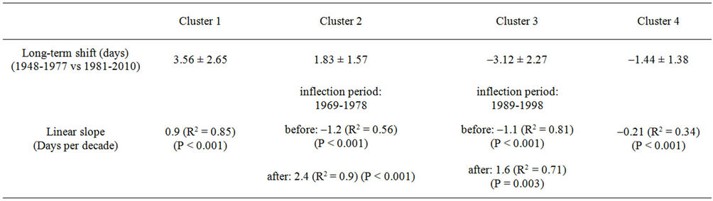
Table 3. Shift of the 1981-2010 temperature cycles in comparison to the 1948-1975 cycles of the clustered areas and the linear trends of the sliding window analyses (α = 0.99).
trends from data collected over less than 30 years is that results highly depend on the chosen period as the shifts change direction over time. Also calculations of large spatial averages are prone to misleading results as phase shifts are heterogeneous on continental and multi-continental scales as shown here (Table 1). Therefore, for the assessment of large area trends in the annual phase shift an appropriate clustering of the observed shifts is required and could be reached with a combination of an SOFM and a k-means algorithm. Four highly significant large-area trends for the globe were found with various directions and even changing directions of the trends over time (Figure 6). This allows a classification of phase shifts of the annual temperature or temporal shifts of phenological events that were observed in many spatially and temporally constricted studies.
The highest long-term phase shifts towards earlier seasons on land from up to –5.5 days over the last 30 years were found in the areas of continental Europe in Belarus and West Russia. Considering the occurrence of such high phase shift values and the effects on the timing of the foliation, coupled climate-carbon cycle models that predict vegetation responses and feedbacks to climate change need to incorporate the effects of the temperature phase shift.
The timing of foliation and hence the ability to assimilate CO2 is highly coupled with the phase shift of temperature. For all of the above reasons, integrating the high resolution spatial and temporal trends and phase shift values presented in this study is an indispensable step for state-of-the-art climate modeling.
5. Acknowledgements
This research was supported by the Office of Science (BER), US Department of Energy. The NCEP/NCAR Reanalysis 1 data was provided by the NOAA/OAR/ ESRL PSD, Boulder, Colorado, USA, from their internet site at http://www.esrl.noaa.gov/psd/data/gridded/data.ncep. rea nalysis.html. The climate report data of the NOAA National Climatic Data Center is available at http://ww w.ncdc.noaa.gov/sotc/global. The North American First Leaf and First Bloom Lilac Phenology dataset was provided by the World Data Center for Paleoclimatology, Boulder and the NOAA paleoclimatology program at ftp://ftp.ncdc.noaa.gov/pub/data/paleo/phenology/north_america_lilac.txt. The authors gratefully acknowledge the provision of the data and the easy public access to these outstanding long-term datasets.
REFERENCES
- S. Solomon, D. Qin, M. Manning, Z. Chen, M. Marquis, et al. Eds., “Climate Change 2007: The Physical Science Basi,” Contribution of Working Group I to the 4th Assessment Report of the Intergovernmental Panel on Climate Change, Cambridge University Press, Cambridge, 2007, p. 996.
- J. Hansen, R. Ruedy, J. Glascoe and M. Sato, “GISS Analysis of Surface Temperature Change,” Journal of Geophysical Research, Vol. 104, No. D24, 1999, pp. 30997-31022. doi:10.1029/1999JD900835
- J. Hansen, M. Sato, R. Ruedy, K. Lo, D. W. Lea and M. Medina-Elizade, “Global Temperature Change,” Proceedings of the National Academy of Sciences, Vol. 103, No. 39, 2006, pp. 14288-14293. doi:10.1073/pnas.0606291103
- P. A. Agudelo and J. A. Curry, “Analysis of Spatial Distribution in Tropospheric Temperature Trends,” Geophysical Research Letters, Vol. 31, 2004, Article ID: L22207. doi:10.1029/2004GL020818
- J. Hansen, R. Ruedy, M. Sato and K. Lo, “Global Surface Temperature Change,” Reviews of Geophysics, Vol. 48, No. 4, 2010, Article ID: RG4004. doi:10.1029/2010RG000345
- D. J. Thomson, “The Seasons, Global Temperature, and Precession,” Science, Vol. 268, No. 5207, 1995, pp. 59- 68. doi:10.1126/science.268.5207.59
- M. Mann and J. Park, “Greenhouse Warming and Changes in the Seasonal Cycle of Temperature: Model Versus Observations,” Geophysical Research Letter, Vol. 23, No. 10, 1996, pp. 1111-1114. doi:10.1029/96GL01066
- C. J. Wallace and T. J. Osborn, “Recent and Future Modulation of the Annual Cycle,” Climate Research, Vol. 22, No. 1, 2002, pp. 1-11. doi:10.3354/cr022001
- M. Palus, D. Novotna and P. Tichavsky, “Shifts of Seasons at the European Mid-Latitudes: Natural Fluctuations Correlated with the North Atlantic Oscillation,” Geophysical Research Letter, Vol. 32, 2005, Article ID: L12805.
- A. R. Stine, P. Huybers and I. Y. Fung, “Changes in the Phase of the Annual Temperature Cycle of Surface Temperature,” Nature, Vol. 457, No. 7228, 2009, pp. 435-440. doi:10.1038/nature07675
- C. Qian, C. Fu, Z. Wu and Z. Yan, “The Role of Changes in the Annual Cycle in Earlier Onset of Climatic Spring in Northern China,” Advances in Atmospheric Sciences, Vol. 28, No. 2, 2011, pp. 284-296. doi:10.1007/s00376-010-9221-1
- A. Aasa, J. Jaagus, R. Ahas and M. Sepp, “The Influence of Atmospheric Circulation on Plant Phenological Phases in Central and Eastern Europe,” International Journal of Climatology, Vol. 24, No. 12, 2004, pp. 1551-1564. doi:10.1002/joc.1066
- K. M. De Beurs and G. M. Henebry, “Northern Annular Mode Effects on the Land Surface Phenologies of Northern Eurasia,” Journal of Climate, Vol. 21, 2008, pp. 4257-4279. doi:10.1175/2008JCLI2074.1
- D. J. Kang and H. J. Wang, “Analysis on the Decadal Scale Variation of the Dust Storm in North China,” Science in China Series D, Vol. 48, No. 12, 2005, pp. 2260- 2266. doi:10.1360/03yd0255
- A. Menzel, T. H. Sparks, N. Estrella, E. Koch, A. Aasa, et al., “European Phenological Response to Climate Change Matches the Warming Pattern,” Global Change Biology, Vol. 12, No. 10, 2006, pp. 1969-1976. doi:10.1111/j.1365-2486.2006.01193.x
- T. L. Root, J. T. Price, K. R. Hall, S. H. Schneider and C. Rosenzweig, et al., “Fingerprints of Global Warming on Wild Animals and Plants,” Nature, Vol. 421, 2003, pp. 57-60. doi:10.1038/nature01333
- M. D. Schwartz, R. Ahas and A. Aasa, “Onset of spring starting earlier across the Northern Hemisphere,” Global Change Biology, Vol. 12, No. 2, 2006, pp. 343-351. doi:10.1111/j.1365-2486.2005.01097.x
- D. Dragoni, H. P. Schmid, C. A. Wayson, H. Potter, C. S. B. Grimmond, et al., “Evidence of Increased Net Ecosystem Productivity Associated with a Longer Vegetated Season in a Deciduous Forest in South-Central Indiana, USA,” Global Change Biology, Vol. 17, No. 2, 2011, pp. 886-897. doi:10.1111/j.1365-2486.2010.02281.x
- C. Parmesan, “Influences of Species, Latitudes and Methodologies on Estimates of Phenological Response to Global Warming,” Global Change Biology, Vol. 13, No. 9, 2007, pp. 1860-1872. doi:10.1111/j.1365-2486.2007.01404.x
- A. L. Westerling, H. G. Hidalgo, D. R. Cayan and T. W. Swetnam, “Warming and Earlier Spring Increase Western U.S. Forest Wildfire Activity,” Science, Vol. 18, 2006, pp. 940-943. doi:10.1126/science.1128834
- G. M. Jenkins and D. G. Watts, “Spectral Analysis and Its Applications,” Holden-Day, San Francisco, 1968, p. 525.
- M. B. Priestley, “Spectral Analysis and Time Series,” Academic Press, London, 1981, p. 890.
- T. Kohonen, “Self-Organization and Associative Memory,” 3rd Edition, Springer, New York, 1998, p. 312.
- T. Kohonen, “The Self-Organizing Map,” Proceedings of IEEE, Vol. 78, No. 9, 1990, pp. 1464-1480. doi:10.1109/5.58325
- World Meteorological Organization, “Calculation of Monthly and Annual 30-Year Standard Normals,” World Meteorological Organization, Geneva, 1989.
- World Meteorological Organization, “The Role of Climatological Normals in a Changing Climate,” WCDMPNo. 61, WMO-TD/No. 1377, World Meteorological Organization, Geneva, 2007.
- T. Smith, M. Thomas, R. W. Reynolds, T. C. Peterson and J. Lawrimore, “Improvements to NOAA’s Historical Merged Land-Ocean Surface Temperature Analysis (1880- 2006),” Journal of Climate, Vol. 21, No. 10, 2008, pp. 2283-2296. doi:10.1175/2007JCLI2100.1
- NOAA National Climatic Data Center. http://www.ncdc.noaa.gov/sotc/global
- E. Kalnay, M. Kanamitsu, R. Kistler, W. Collins, D Deaven, et al. “The NCEP/NCAR 40-Year Reanalysis Project,” Bulletin of the American Meteorological Society, Vol. 77, No. 3, 1996, pp. 437-471. doi:10.1175/1520-0477(1996)077<0437:TNYRP>2.0.CO;2
- The NOAA Earth System Research Laboratory, Physical Science Division. http://www.esrl.noaa.gov/psd/data/gridded/data.ncep.reanalysis.html
- R. Kistler, E. Kalnay, W. Collins, S. Saha, G. White, et al., “The NCEP–NCAR 50-Year Reanalysis: Monthly Means CD-ROM and Documentation,” Bulletin of the American Meteorological Society, Vol. 82, No. 2, 2001, pp. 247-267. doi:10.1175/1520-0477(2001)082<0247:TNNYRM>2.3.CO;2
- D. Barriopedro, E. M. Fischer, J. Luterbacher, R. M. Trigo and R. García-Herrera, “The Hot Summer of 2010: Redrawing the Temperature Record Map of Europe,” Science, Vol. 332, No. 6026, 2011, pp. 220-224. doi:10.1126/science.1201224
- X.-Z. Wang, M. Yoshizawa, A. Tanaka, K. Abe, K. Imachi, et al., “An Automatic Monitoring System for Artificial Hearts Using a Hierarchical Self-Organizing Map,” The International Journal of Artificial Organs, Vol. 4, No. 3, 2001, pp. 198-204. doi:10.1007/BF02479894
- N. Tigrine-Kordjani, F. Chemat, B. Y. Meklati, L. Tuduri, J. L. Giraudel, et al., “Relative Characterization of Rosemary Samples According to Their Geographical Origins Using Microwave-Accelerated Distillation, Solid-Phase Micro Extraction and Kohonen SelfOrganizing Maps,” Analytical and Bioanalytical Chemistry, Vol. 389, No. 2, 2007, pp. 631-641. doi:10.1007/s00216-007-1441-6
- U. S. N. Murty, A. K. Banerjee and N. Arora, “Application of Kohonen Maps for Solving the Classification Puzzle in AGC Kinase Protein Sequences,” Interdisciplinary Sciences Computational Life Sciences, Vol. 1, No. 3, 2009, pp. 173-178. doi:10.1007/s12539-009-0032-1
- A. Schmidt, C. Hanson, J. Kathilankal and B. E. Law, “Classification and Assessment of Turbulent Fluxes above Ecosystems in North-America with Self-Organizing Feature Map Networks,” Agricultural and Forest Meteorology, Vol. 151, No. 4, 2011, pp. 508-520. doi:10.1016/j.agrformet.2010.12.009
- E. Arsuaga-Uriarte and F. Diaz-Martin, “Topology Preservation in SOM,” International Journal of Applied Mathematics and Computer Science, Vol. 1, No. 1, 2005, pp. 19-22.
- D. L. Davies and D. W. Bouldin, “A Cluster Separation Measure,” IEEE Transactions on Pattern Analysis and Machine Intelligence, Vol. 1, No. 2, 1979, pp. 224-227. doi:10.1109/TPAMI.1979.4766909
- A. K. Jain and R. C. Dubes, “Algorithms for Clustering Data,” Prentice Hall, Englewood Cliffs, 1988, p. 334.
- U. Maulik and S. Bandyopadhyay, “Performance Evaluation of Some Clustering Algorithms and Validity Indices,” IEEE Transactions on Pattern Analysis and Machine Intelligence, Vol. 24, No. 12, 2002, pp. 1650-1654. doi:10.1109/TPAMI.2002.1114856
- L. B. Webb, P. H. Whetton and E. W. R. Barlow, “Observed Trends in Winegrape Maturity in Australia,” Global Change Biology, Vol. 17, No. 8, 2011, pp. 2707- 2719. doi:10.1111/j.1365-2486.2011.02434.x
- J. A Carton and Z. Zhou, “Annual Cycle of Sea Surface Temperature in the Tropical Atlantic Ocean,” Journal of Geophysical Research, Vol. 102, No. C13, 1997, pp. 27813-27824. doi:10.1029/97JC02197
- P. Knudsen, O. B. Andersen and T. Knudsen, “Annual Cycles of ERS-1 Altimetric Sea Surface Height Data and ATSR Sea Surface Temperature Data,” 3rd ERS Symp. on Space at the Service of our Environment, Florence, 17-21 March 1997.
- M. D. Schwartz, “Monitoring Global Change with Phenology: The Case of the Spring Green Wave,” International Journal of Biometeorology, Vol. 38, No. 1, 1994, pp. 18- 22. doi:10.1007/BF01241799
- M. D. Schwartz and B. E. Reiter, “Changes in North American Spring,” International Journal of Climatology, Vol. 20, No. 8, 2000, pp. 929-932. doi:10.1002/1097-0088(20000630)20:8<929::AID-JOC557>3.0.CO;2-5
- D. R. Cayan, S. A. Kammerdiener, M. D. Dettinger, J. M. Caprio and D. H. Peterson, “Changes in the Onset of Spring in the Western United States,” Bulletin of the American Meteorological Society, Vol. 82, No. 3, 2001, pp. 399-415. doi:10.1175/1520-0477(2001)082<0399:CITOOS>2.3.CO;2
- T. Imaizumi and S. A. Kay, “Photoperiodic Control of Flowering: Not Only by Coincidence,” Trends in Plant Science, Vol. 11, No. 11, 2006, pp. 550-558. doi:10.1016/j.tplants.2006.09.004
- J. Repkova, M. Brestic and K. Olsovska, “Leaf Growth under Temperature and Light Control,” Plant, Soil and Environment, Vol. 55, No. 12, 2009, pp. 551-557.
- B. Min, “Comparison of Phenological Characteristics for Several Woody Plants in Urban Climates,” Journal of Plant Biology, Vol. 43, No. 1, 2000, pp. 10-17. doi:10.1007/BF03031030
- J. Vesanto and E. Alhoniemi, “Clustering of the SelfOrganizing Map,” IEEE Transactions on Neural Networks, Vol. 11, No. 3, 2000, pp. 586-600. doi:10.1109/72.846731
NOTES
*Corresponding author.