Journal of Signal and Information Processing
Vol. 3 No. 1 (2012) , Article ID: 17666 , 14 pages DOI:10.4236/jsip.2012.31009
Interactive Kalman Filtering for Differential and Gaussian Frequency Shift Keying Modulation with Application in Bluetooth
![]()
Electrical and Computer Engineering Department, Oakland University, Rochester, USA.
Email: {mnali, zohdyma}@oakland.edu
Received November 11th, 2011; revised December 13th, 2011; accepted December 26th, 2011
Keywords: Interactive Kalman Filtering; Unscented Kalman Filter; Extended Kalman Filter; Differential Quadrature Phase Shift Keying; Gaussian Frequency Shift Keying; Bluetooth
ABSTRACT
Some applications are constrained only to implement low cost receivers. In this case, designers are required to use less complex and non-expensive modulation techniques. Differential Quadrature Phase Shift Keying (DQPSK) and Gaussian Frequency Shift Keying (GFSK) can be non-coherently demodulated with simple algorithms. However, these types of demodulation are not robust and suffer from poor performance. This paper proposes a new method to enhance the performance of DQPSK and GFSK using Interactive Kalman Filtering (IKF) technique, in which a one Unscented Kalman Filter (UKF) and two Kalman Filters (KF) are coupled to optimize the demodulated signals. This method consists of simple but very effective algorithms without adding complexity to the demodulators comparing to other very complex methods. UKF is used in this method due to its superiority in approximating and estimating nonlinear systems and its ability to handle non-Gaussian noise environments. The proposed method has been validated by creating a MATLAB/SIMULINK Bluetooth system model, in which the IKF is integrated into the receiver, which implement both DQPSK and GFSK, and run simulation in Gaussian and Non-Gaussian noise environments. Results have shown the effectiveness of this method in optimizing the received signals, and that the UKF outperforms the Extended Kalman Filter (EKF).
1. Introduction
Receivers with noncoherent demodulation have simple structures, but they don’t have robust performance [1-3]. Simple noncoherent demodulators are attractive in applications where cost is a concern. For example, in Bluetooth protocols [4], noncoherent detection of GFSK and variants of Differential Phase Shift Keying (DPSK) are specified due to their simplicity and low costs. Although these non-optimal techniques are sufficient in low noisy channels, they may suffer performance degradations in very noisy environments.
In order to optimize the performance of the noncoherent demodulation, some complex Maximum Likelihood Sequences Estimator (MLSE) is utilized. An efficient method of implementing this estimation process is through the usage of the very complex Viterbi algorithm that searches the paths through the state trellis for the minimum Euclidean distance path [1]. It was shown that using the Viterbi decoder in Bluetooth receiver achieved very superior performance, but added more complexity, comparing to the noncoherent demodulation that consists of Limited Discriminator with integrating and dump filter [5].
DQPSK is one form of DPSK. It is a memoryless, and a discontinuous phase modulation, in which the current binary sequence is modulated independently of the previous sequences. GFSK is a subclass of Continuous Phase Modulation (CPM), and an attractive modulation in many applications due to its enhanced spectral properties. In modulations, where phase is not continuous, poor spectral efficiency is a real issue. Discontinuities and abrupt changes in phase cause this poor performance, making CPM a more favored scheme [2,6]. GFSK is a modulation with memory, in which the current transmitted signal depends on the current and previous binary sequences. In DQPSK, the phase is constant over a one symbol interval, while in GFSK the phase varies continuously over the symbol period [7]. Both DQPSK and GFSK can be detected non-coherently, which results in simplified transceivers [8].
In the latest Bluetooth specifications, two types of modulation schemes are specified. The first one is the GFSK, which is a form of Continuous Phase Frequency Shift Keying (CPFSK), and hence CPM [9]. It is used in the Basic Data Rate (BDR), with transmission rate at 1 Mbps. The other type is the Differential Phase Shift Keying (DPSK), which is used in the Enhanced Data Rate (EDR) with two variants, π/4-DQPSK and 8DPSK. The transmission rates are 2 Mbps for EDR using π/4-DQPSK and 3 Mbps using 8DPSK [4]. Data are transmitted in frames of 625 µs time slots. Each frame is divided mainly into Access Codes (AC) and Payloads. In the EDR, the AC is modulated using one of the DPSK variants, while the payload is modulated using GFSK. No equalization requirements are specified in Bluetooth protocols in order to preserve the low complexity of the system, leaving this area open for researchers to propose efficient equalization and optimization methods that improve the performance of the system, but without inducing much costs.
Significant amount of researches have been conducted to optimize the performance of the DQPSK and GFSK noncoherent demodulation. A. Soltanian and R. E. Van Dyck showed that in typical Bluetooth indoor applications, the noncoherent limiter-discriminator with integrate and dump filter receiver, without equalization, achieves reasonable performance; but this is not the case for the outdoor and large indoor applications, where the signal needs to be more robust. They suggested the usage of Viterbi receiver to get optimum results for such applications [5]. In [9], N. Ibrahim, L. Lampe, and R. Schober presented a receiver design for a GFSK demodulator based on Laurent’s decomposition. They developed a Non-coherent Decision Feedback Equalizer (NDFE) and showed that it achieved a robust performance comparing to other equalization methods. In their method, they handled the nonlinearity in the modulation by transforming it into linear using Laurent’s decomposition.
M. Nafie, A. Gatherer, and A. Dabak presented a nonadaptive a fractionally sampled Decision Feedback Equalizer (DFE) to be added after the discriminator to enhance the performance of noncoherent GFSK receivers. The proposed DFE was non-adaptive, and they proposed this equalizer to be trained off line at a certain SNR and then this will be used in reception [10]. Harry Leib presented his work that considered an optimal noncoherent demodulation of DPSK when the receiver has partial knowledge of the transmitted data. They proposed A Maximum Likelihood (ML) noncoherent receiver in [11]. The same technique was implemented for GFSK signals in [12].
Implementing Kalman Filtering to enhance the performance of noncoherent continuous and differential phase demodulation have been proposed in several articles. In [13,14], Gal, Campeanu, and Nafornita proposed a method of applying Extended Kalman Filtering in the noncoherent demodulation of CPM and CPFSK respectively. In [15], O. Loffeld utilized the EKF in the demodulation of noisy phase or frequency of sinusoidal signals of unknown amplitude in the presence of an Additive Wideband Gaussian Noise (AWGN). He assumed that the state space model of the unknown phase and amplitude were known. Those Proposed papers utilized linearization technique on the system before using the EKF.
In 1960, Rudolf E. Kalman presented his Kalman Filter method in [16]. KF is an estimator, in which it estimates the states in linear dynamic systems by minimizing the Minimum Mean Squared Error (MMSE). Kalman invented this based on modifying Wiener-Kolmogorov filter, which was derived in 1940 [17]. KF is originated from Baye’s probabilistic theory, in which if good number of past samples are known, the future samples can be predicted and updated based on the continuously collected results [18]. Techniques have been proposed to modify KF to be applied to nonlinear systems. For example, EKF has been proposed in nonlinear systems estimations by linearizing the estimated variables through deriving Jacobian matrices. However, EKF may not be a good choice in system with high nonlinearity, or systems that are very difficult to calculate their Jacobian matrices [19].
All the referenced techniques as mentioned thus far are either very complex, or suffer from inadequacy in handling nonlinearly and non-Gaussian noise environments. A better method to approximate nonlinear systems and apply Kalman filtering equations to them was proposed by S. Julier and J. Uhlmann [20]. UKF was derived based on the unscented transformation (UT) concept, which is used to approximate random variables distributions that are going through nonlinear transformations without a need to calculate the probability density functions (pdf) of the nonlinearly transformed variables. UKF has been demonstrated to be very effective in applications when dealing with nonlinear dynamic systems and non-Gaussian types of noises comparing to other filtering techniques [21]. Several types of UKF methods have been developed based on different techniques of UT. These techniques include the General Unscented Transformation, the Scaled Unscented Transformation, the Reduced Sigma Point, and the Spherical Simplex Unscented Transformation [22-25]. In [26], M. Ali and M. Zohdy proposed using UKF in the equalization of CPFSK. They showed that UKF outperformed EKF when both implemented in the CPFSK.
In this paper, we are proposing the implementation of IKF to enhance the performance of the noncoherent demodulation of DQPSK and GFSK. It will be shown that UKF has superior performance in approximating nonlinear systems, and in handling non-Gaussian noise than the already existed EKF methods. This proposed method is an attractive one in the sense that it has simple algorithms so that not that much complexity is added to the receivers comparing to the optimum demodulation. Simulation will be run on a developed MATLAB/SIMULINK model representing Bluetooth system. Results will be compared to those generated by the same model before the implementation of this method, and when using EKF.
This paper has been organized as follow. Introduction is presented in the Section 1. Section 2 will details the new method of the unscented transformation, and how to apply it in UKF. Section 3 will discuss the signal descriptions of DQPSK and GFSK, and Section 4 will detail the system models of both. Section 5 will explain the IKF algorithms. In Section 6, the simulation and results will be listed. Section 7 lists the conclusion.
2. Unscented Transformation and Unscented Kalman Filter
The UT does not approximate the nonlinear process and observation functions. It approximates the statistics (mean and covariance) of the state variable ![]() which has dimension
which has dimension  by carefully choosing a deterministic set of sample points
  and their corresponding weights
 which have dimensions
 . These sigma points and their associated weights are chosen carefully to capture accurately the actual mean and covariance of the state variables, and when the sampled mean and covariance are propagated through a nonlinear system
 , the a posteriori mean and covariance of the state variables can be estimated accurately up to the 3rd order of any nonlinearity [20]. The statistics of the random variables can also be approximated for higher nonlinearity (4th order and up) but with some errors. Figure 1 illustrates the principle behind the UT when some deterministic points are undergoing nonlinear transformation.
2.1. Choosing Sigma Points
There is no single method of choosing sigma points that guarantees global optimization of a system. Rather, many methods have been proposed in which each one has advantages and disadvantages over the others. Simon Julier proposed the Scaled Unscented Transformation (SUT) in [23] to be able to control the sigma points without the possibilities of the covariance to become non-positive semi-definite. In the SUT, the sigma points are calculated as follow:
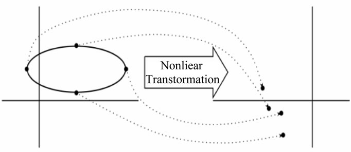
Figure 1. Nonlinear transformations using unscented transformation.
 (1)
(1)
where, 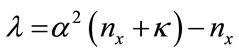 , and
, and  and
and  are the associated weights of these sigma points. The scaling factor
  is a tool to scale the sigma points towards or away from the mean. It should be noted that there is no general way to propose the values of the scaling factors
 . In each application, these values should be chosen to reduce the estimation errors for their specific problems. As an example, for Gaussian distributions, the scaling factors
  can be set to 2, 0.001, and 0 respectively for optimum estimation [21].
2.2. The Unscented Kalman Filtering
The UKF is a novel method that was proposed in [20] to propagate the mean and covariance of a random variable through nonlinear systems using the unscented transformation in order estimate the a posteriori mean and covariance. The following lists the steps for the UKF algorithm based on the SUT.
2.2.1. Nonlinear System Equations
A nonlinear system can be represented as:
 (2)
(2)
 (3)
(3)
Equation (2) models the system process model, where  represents the states to be estimated,
  represents the input, and
  represents the process noise that has zero mean and covariance
 . Equation (3) models the observation model, where
  represents the measurement noise, which has zero mean and covariance
 .
.
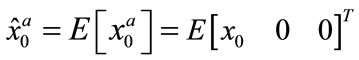
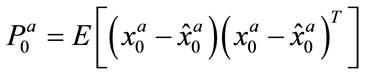
2.2.2. Initialization and Sigma Points Calculation
The state vector and process covariance matrix need to be initialized as follow:
 (4)
(4)
 (5)
(5)
where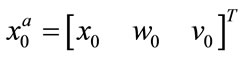 . Equation (1) can be used to derive
  deterministic sigma points, which can be written as:
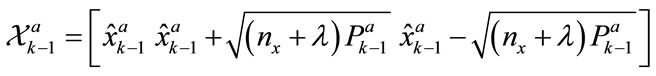 (6)
(6)
2.2.3. Time Update Equations
The sigma points in Equation (6) are propagated through the nonlinear process function in Equation (2) to give:
 (7)
(7)
The sampled predicting mean and covariance of the state variable are calculated in the next two equations.
 (8)
(8)
 (9)
(9)
2.2.4. Measurement Update Equations
In order to derive the measurement update equations, the sigma-point states as derived in Equation (7) need to be propagated in the nonlinear measurement model in Equation (3).
 (10)
(10)
The output sampled mean and covariance are captured as follow:
 (11)
(11)
 (12)
(12)
The cross covariance of the state and measurement can be calculated as:
 (13)
(13)
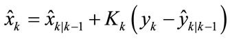
Using the conventional KF equations, we can calculate Kalman gain as:
 (14)
(14)
where,  and
and  are derived in Equations (12) and (13) respectively. The Kalman gain as derived in Equation (14) can be used in the following equation to calculate the updated a posteriori mean of the states.
 (15)
(15)
Finally, the update covariance can be expressed as:
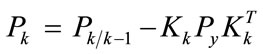 (16)
(16)
3. π/4 DQPSK and GFSK Signal Description
3.1. π/4 DQPSK Signal Description
The π/4-DQPSK is a version of DQPSK, but shifted by π/4. For simplicity we refer to π/4-DQPSK as DQPSK throughout this paper. Its transmitted signal can be represented as [27]:
 (17)
(17)
where represents the carrier-modulated signal,
  is the information-carrying phase that mapped to a symbol
 ,
,  and
and  are the symbol energy and duration respectively.
  and
and  is the number of symbols, which is 4 in the case of DQPSK. At
  the dynamic behavior of the phase can modeled as:
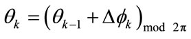 (18)
(18)
where the addition is modulo .
.  is the value, which results from mapping the binary sequences to the phase representation. Thus, 11, 01, 00, 10 sequences are mapped to
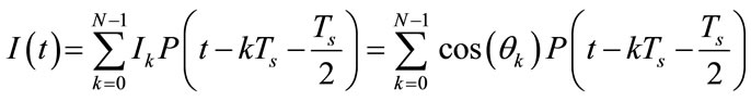
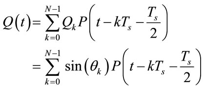
 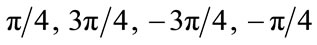 respectively. Equation (18) shows the dynamic transition when phase is changing from current transmitted symbol to the next one. The Inphase
  and Quadrature
  components (complex envelops) of the transmitted signal of the
  symbol are determined as follow:
 (19)
(19)
 (20)
(20)
The Inphase  and Quadrature
  are functions of the phase
  which is in turn functions of the previous state
  and the current input
 . This is modulated this way so that the only information needed at the demodulator side is the difference between the consecutive received phases, which enable simpler noncoherent demodulation. The In-phase and Quadrature are passed through pulse shape filters to smooth the pulses and conserve the bandwidth. When pass through these filters, the resulted pulses are represented as:
 (21)
(21)
 (22)
(22)
There are several forms of the pulse shapes , which can take the forms of Gaussian, Raised Cosine, and others. When these components are multiplied by the carrier, the resulted baseband modulated signal is:
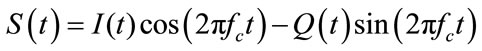 (23)
(23)
3.2. GFSK Signal Description
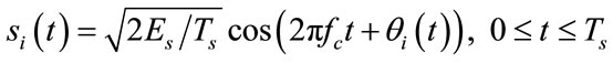
The transmitted carrier-modulated GFSK signal can be represented in the following format [12,27]:
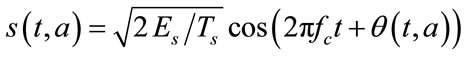 (24)
(24)
The complex baseband waveform of this signal can be expressed as:
 (25)
(25)
where the phase can be represented as:
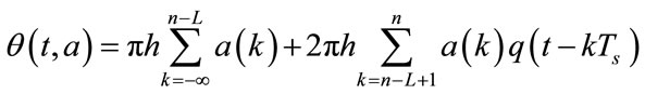 (26)
(26)
where ,
,  represents the carriermodulated signal,
  is the time-varying phase of the carrier,
  is the symbol energy,
  is the symbol duration, and
  is the carrier frequency. The digital sequence
  represents the M-ary information symbols that can take the following symbol format
 , and for binary sequences,
 . h is the modulation index. The first term on the right side of Equation (26) models the phase history.
  is the phase response, which is derived by integrating a pulse
 , and
, and  is the length of this pulse (per unit
 ).
).  is defined as the instantaneous frequency of
 . The shape of
  determines the smoothness of the transmitted carrying information phase [28]. For example, in the case of GFSK,
  is shaped using Gaussian pulses instead of rectangular as this the case in CPFSK. There are Different pulse shapes, such as Raised Cosine (RC), and Gaussian Minimum Shift Keying (GMSK), etc.
4. π/4 DQPSK and GFSK System Description
In Kalman Filtering, two steps are performed; prediction and update. It is important that the received signal to be predictable in order to use Kalman Filters. Thus, the system under study needs to be modeled to allow performing prediction. Both DQPSK and GFSK dynamic systems will be modeled nonlinearly, and transformed into state space format so that Kalman filtering can be applied. In the noncoherent DQPSK, the current phase is a function of the previous phase and the current input, making it possible to do the prediction task of the next phase. In the case of GFSK, or any other CPM, Kalman Filtering can be an attractive technique since the transition in phase is continuous, and the changes do not occur abruptly, making the prediction step possible also.
4.1. π/4 DQPSK Dynamic System Description
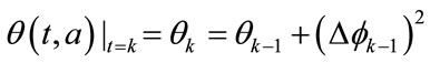
Before the signal goes through decoding and decision state, it goes through the proposed Interactive Kalman Filtering for optimization. In order to apply Kalman Filtering, we need first to derive the state space equations that describe the system. The RC shaping pulse  causes the phase response
  to be nonlinear. Therefore, at
 , the phase can be represented nonlinearly using Euler’s formula as:
 (27)
(27)
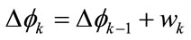
where the delta change  representing the change from one phase to the next one can be approximated as:
 (28)
(28)
Equation (28) is the first order difference equation of the phase.  is a discrete value and constant over one symbol duration.
  represents the symbol sequences, and
  is the process noise, which is assumed to have zero mean and variance
 .
.  is the step size, which is treated as a fixed number in this paper, that determines the change value from
  to
to . The smaller this value is, the smaller the nonlinear approximation error is.
  is the rate of the change (slope) at
 . If a rectangular pulse shape
  was considered as it is the case in CPFSK, than equation (27) can be modeled linearly as
 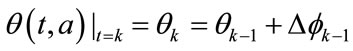 [13]. However, for GFSK, this behavior is nonlinear, and Equation (27) can be represented as:
 (29)
(29)
4.1.1. State Transition Model
There are two states in the system, the phase  and the difference equation
  that need to estimated. The following equations represent the dynamic system of the DQPSK in state space format.
 (30)
(30)
 (31)
(31)
These can be written in the following matrix format:
 (32)
(32)
In order to calculate , some a priori knowledge of
  at
at  is needed. Thus, Equation (28) can be re-written as:
 (33)
(33)
where  is the prediction of the phase at
  having knowledge of the phase up to
 .
.  can be estimated using two coupled Kalman Filters, as it will be explained in Section 5.
4.1.2. Measurement Models
When transmitted through an ideal channel, which is corrupted by AWGN, the Inphase and Quadrature components of the received signal at  can be represented as:
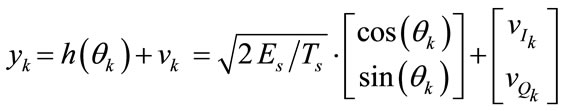 (34)
(34)
where  and
and  are the measurement noise of the Inphase and Quadrature components respectively.
4.2. GFSK Dynamic System Description
GFSK is different from the DQPSK in a sense that it is a frequency shift keying modulation, and its phase is changing continuously during a symbol transmission [7]. There are two states to estimate in this system, the continuously changing phase  and the difference equation
 , where
  is the input sequences. The dynamic equations can be represented as:
 (35)
(35)
 (36)
(36)
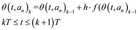
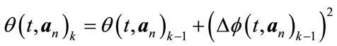
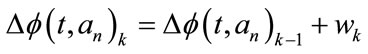
Equation (35) states that when the state changes from  to
to over a symbol
  with duration
 ,
,  can be determined using Euler’s formula by adding the change in the phase
  to the previous phase
 .
.  is the step size, and
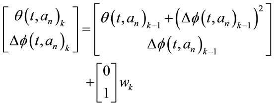
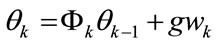
  is the process noise. This dynamic system can be modeled nonlinearly as:
 (37)
(37)
At the receiver, the signal can be modeled as:
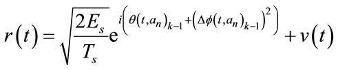 (38)
(38)
where .
.
4.2.1. State Transition Model
The dynamic system of the phase and difference equation of the GFSK can be written as:
 (39)
(39)
 (40)
(40)
In a matrix format, (39) and (40) can be represented as
 (41)
(41)
4.2.2. Measurement Model
When transmitted through an ideal channel with AWGN, the Inphase and Quadrature components of the received signal at  can be represented as:
 (42)
(42)
4.3. π/4 DQPSK and GFSK Dynamic System Description
There are communication systems that implement multiple modulation schemes, such as WIFI, Bluetooth, etc. Figure 2 represents a receiver that implements both DQPSK and GFSK, similar to the modulation schemes as specified in Bluetooth communications [4]. This figure depicts a functional blocks of the demodulator along with the proposed IKF interface. The DQPSK part of the demodulator processes the AC and Headers portion of the frames, while the GFSK part of the demodulator processes the Payloads portion of the frames. As it will be explained in the next section, the two KFs calculate the a priori phase  and feed it into the UKF. In its turn, UKF uses this a priori and knowledge of the noise characteristics, and apply its simple algorithms to estimate the received signal components, before it feeds it into the decoding and decision devices for further processing.
Next, the state space equations for both DQPSK and GFSK systems are presented, which include 4 states, and 4 outputs.

Figure 2. The baseband DQPSK and GFSK receiver with the integrated Kalman filtering.
4.3.1. State Transition Model
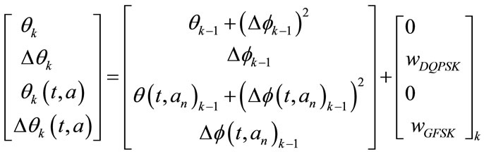 (43)
(43)
4.3.2. Measurement Model
The measurement equations can be written as follow:
 (44)
(44)
5. Interactive Kalman Filtering
Dual estimations concept has been explored in several researches in different applications. In [29], D. Labarre et al. proposed to take advantage of the so-called instrumental variable (IV) techniques to estimate both the received signal and the associated parameters. They proposed using two conditionally linked Kalman Filters in order to avoid using an EKF to estimate both states and parameters. The first KF uses a new observation to estimate the incoming signal, while the second KF uses this estimated signal to estimate the coefficient parameters. In [30], A. Jamoos, A. Abdo, and H. Nour used similar technique to jointly estimate channel coefficients and parameters using two coupled Kalman Filters in the estimation of rapidly time-varying Rayleigh fading channels in Orthogonal Frequency Division Multiplexing (OFDM) mobile wireless system. Thus, each time a new observation is available, the first filter uses the latest estimated parameters to estimate the signal, while the second filter uses the estimated signal to update the parameters.
5.1. Phase Prediction
This joint estimation method will be utilized to predict the a priori phase  based on the past measured received signals
 , and feed this predicted value into in UKF to use it in its algorithm. From Equation (29), the phase
  is predicted based on the previous value
  and the change as triggered by the current input, which is equivalent to
 . Thus, in order to calculate
 , we need to have knowledge of
 . At the mean time, we need to know
  in order to calculate
 . The dual estimation is proposed to handle this case to predict the phase
 . The phase
  is replaced by
  in Equation (29), which can be written as:
 (45)
(45)
This a priori can be predicted recursively using the following formula:
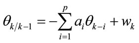 (46)
(46)
where  is the prediction coefficients,
  is the so called driving process and it is assumed to be zero-mean noise with variance
 , and
, and  is the order. This is called joint estimation [18], since both the phase
  and their coefficients
  need to be estimated, and they depend on each others. Two KFs are proposed in order to perform the estimation, which allow the analysis to be run linearly and avoid using any of the nonlinear approximation methods.
KF1 estimates the phases, while KF2 estimates their coefficients. Figure 3 shows a layout of this proposed IKF method.
5.2. Estimation of the Phase Values
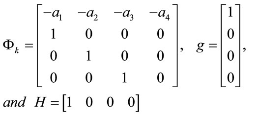
Let . Equation (46) can be put in the following state space format:
 (47)
(47)
 (48)
(48)
When , these matrices are defined as:
The goal is to estimate the phase  at
at , given
  observations of
  as well as estimating the output
  also. The a posteriori
  is defined as:
 (49)
(49)
where,  is called innovation process and is defined as
 . Its covariance can be defined as:
 (50)
(50)
The so called a priori error covariance matrix  can be calculated recursively as:
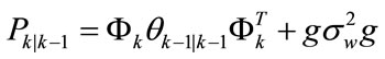 (51)
(51)
 is called the Kalman gain, and is calculated as:
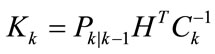 (52)
(52)
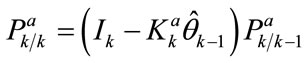
The so called a posteriori covariance is updated as follow:
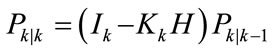 (53)
(53)
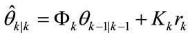
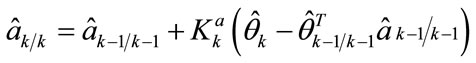
Finally, the output of KF1 is the predicted phase and can be expressed as:
 (54)
(54)
The estimated phase  will be fed into KF2 as the observed values and used in the coefficients estimation, and
  will be used as the a priori
  and fed into the UKF. The state vector and its covariance can be initialized as
  and
and .
.
5.3. Estimation of the Coefficients
The state vector  that was estimated in KF1 is used
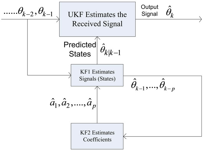
Figure 3. Interactive Kalman filtering.
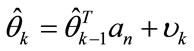
as the observed value to KF2. In order to estimate the coefficients from the estimated phase, Equations (49) and (54) are combined as:
 (55)
(55)
For the 4th order system, the phase and coefficients vectors are defined as 
and  respectively. Assuming that the phase signal is stationary or changing very slowly from the current value to the next one, it is possible to assume that the coefficients to be approximately time invariant over a short period of time. In this case they can be written as:
 (56)
(56)
Now we are ready to define the state space equations for KF2 to estimates the coefficients as:
 (57)
(57)
 (58)
(58)
where  become the observed values, and
  are the states to be estimated. The covariance of the process
  can be calculated as:
 (59)
(59)
The coefficients can be recursively computed as:
 (60)
(60)
where the Kalman gain  and the update state covariance matrix
  can be calculated as:
 (61)
(61)
 (62)
(62)
In the same manner, the initial state and its covariance can be initialized as:  and
and .
.
6. Simulation and Results
6.1. MATLAB/SIMULINK Bluetooth Model
A Bluetooth model has been created to implement and validate the proposed method. This model was created in the MATLAB/SIMULINK environments [4]. The transmitted signal power is set to 100 mw representing Bluetooth class 1 devices, which can communicate up to 100 meters. The model consists of three parts; the transmitter, the channel, and the receiver. In the transmitter, the data go through the source and channel coding. The data are structured in frames. In the simulation runs, data representing actual speech signals have been processed. Data are organized in frames. Each frame contains 72 bits for Access Codes (AC), 56 bits for Headers, and 240 bits for the payloads, which makes up a total of 366 bits per frame. The 126 bits representing the AC and Headers are modulated using  DQPSK in this model, and the 240 bits are modulated with GFSK, and transmitted over an AWGN channel in 625 µs time slots. In some of the simulation runs, non-Gaussian channel was used.
The receiver was simulated so that the frame was divided into two sections. The first section is processed by the  DQPSK portion of the demodulator (bits 1 - 126), while the other sections was build with the GFSK demodulator to process bits 127 - 366. The rest of the blocks in the receiver were simulated to perform all required decoding, and reconstructing of the source signal. The proposed IKF was integrated into the receiver to estimate and optimize the received signals. Figure 4
shows a high level schematic of this model.
At the receiver, the corrupted signal goes through the IKF with UKF or EKF to perform the estimation steps on it before feeding it into the demodulator. Figure 5 shows schematic of the integrated IKF, which include the 2 KFs and a UKF as implemented in the receiver. It also includes the blocks to calculate the un-filtered phase and the UKF estimated phase, and their associated MSE.
6.2. Results
Simulation was run to compare the performance of the system with the integrated IKF versus the same system model without Kalman Filtering. Also, the performances of both the UKF and EKF were compared. Figure 6 shows the results when 200 samples of the received signal were plotted for non-filtered versus the IKF estimated signals, which consists of two KFs and one UKF. The non-noisy transmitted signal was used as a reference. Plots show clearly that IKF improves the signals significantly over the non-enhanced receiver. In the simulation, the SNR was set at value 10. This result shows the advantages of using simple algorithm like IKF to improve the results.
Figure 7 shows the corresponding Square Error (SE), of the un-processed (non-filtered) received signal versus the SE of the IKF estimated signal. These SE values were calculated in reference to the transmitted (non-noisy) signals for the same 200 samples as in Figure 6. Results have been consistent in showing that the implementation of IKF has improved the received signal significantly and consistently in enhancing the noncoherent modulation per-
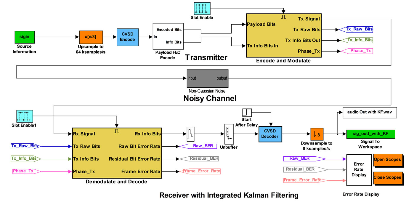
Figure 4. Bluetooth system model with the integrated interactive Kalman filtering in the demodulator.
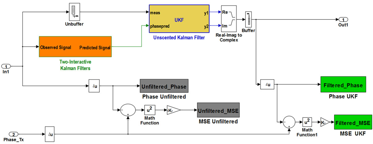
Figure 5. The integrated Kalman filtering as implemented in the bluetooth receiver model.
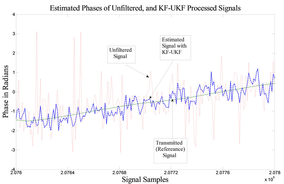
Figure 6. Non-filtered signal versus IKF estimated signals.

Figure 7. Square error of the non-filtered and IKF estimated signals.
formance.
Figure 8 shows the normalized MSEs of the non-estimated, estimated EKF, and UKF signals, when both filters implemented using the proposed IKF method in Bluetooth systems with DQPSK & GFSK modulation in the presence of Gaussian noise. The results show that the both EKF and UKF improve the signals significantly when comparing the results to the receivers with no filtering. It also shows that UKF outperforms the EKF for all SNR values from 0 to 12.
Non-Gaussian noise distributions can be modeled as a mixture of additive zero-mean Gaussians distributions [31]. In [32], L. Binh used SIMULINK to simulate nonGaussian noise as a mix of Gaussian distributions. Figure 9 shows that UKF continues to outperform the EKF in the presence of non-Gaussian noise, which was created by adding three zero mean Gaussian noise distributions using SIMULINK built-in blocks.
When the step size  in Equations (29) and (35) became smaller, modeling errors would be smaller, enabling modeling the system more accurately for Kalman

Figure 8. Normalized MSEs of the non-estimated, estimated EKF, and estimated UKF in the presence of Gaussian noise.

Figure 9. Normalized MSEs of the non-estimated, and estimated EKF and UKF in the non-Gaussian noise.
Filters, which results in better estimation. This is an expected behavior, since with smaller step size the change from the current sample to the next one will be smaller, enabling KF to do more accurate prediction and update. Controlling this processing step size at the demodulator can be done by taking more or less samples per symbol. When taking more samples over the duration of the symbol, this results in smaller step size. Figure 10 shows clearly the comparison of the BER when the UKF was used in the IKF with 0.01 versus when this step size was doubled to be 0.02. Results show that choosing smaller step size results in much better performance. However, the disadvantage of smaller step size is that more computations are needed.
Figures 7-10 simulated the performance when using both DQPSK and GFSK modulation in the simulated Bluetooth system model. The following figure represents performance when only DQPSK is used. Figure 11 shows the simulation when the signals were UKF estimated signals for three values of the step size. In the first case, step size was chosen to be 1. The second and third step sizes were chosen to be 0.125 and 0.0625 to represent

Figure 10. BER of the DQPSK and GFSK demodulated signal when step size was chosen to be 0.01 and 0.02.
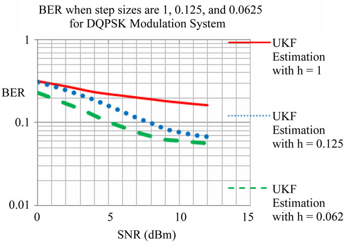
Figure 11. BER of the DQPSK demodulated signal when step sizes were chosen to be 1, 0.125, and 0.0625.

Figure 12. The estimated signals and associated square errors of the UKF and EKF for GFSK modulated signals.
when 8 and 16 samples per symbol respectively.
When GFSK were the only modulation impeleneted in the Bluetooth system model as in the BDR, and simulation trials were run to compare the UKF and EKF performance, results were consistent in showing the superiroity of the UKF. Figure 12 shows the comparison between the EKF and UKF estimated signals for both the phase signlas, and the associated SE. Results show clearly that UKF continues to produce bettr results than EKF.
For the GFSK only modulation system model, and in order to show that our proposed method is consistent over different types of randomly generated noises, we have run 10 simulation experiments for each SNR. Thus, for each SNR value, simulation has been run 10 times, using different values of noise seeds to generate different results in each trial. A total of 100 runs were executed, and when calculating the average of their MSEs, results showed clearly that UKF outperforms the EKF. The results, as they are shown in Table 1 below, reveal the outcomes of these experiments.
7. Conclusion and Future Work
In this paper, a novel IKF method has been proposed to optimize the performance of the non-coherent demodulation of DQPSK and GFSK. The results have demonstrated that this method is an effective when implemented in both modulation schemes, while preserving their simple structures. UKF has been proposed to be used in these digital modulation schemes, and has proven to be robust in handling the nonlinearity of both schemes and when operating in non-Gaussian noise environments. Utilizing UKF in DQPSK and GFSK has been validated
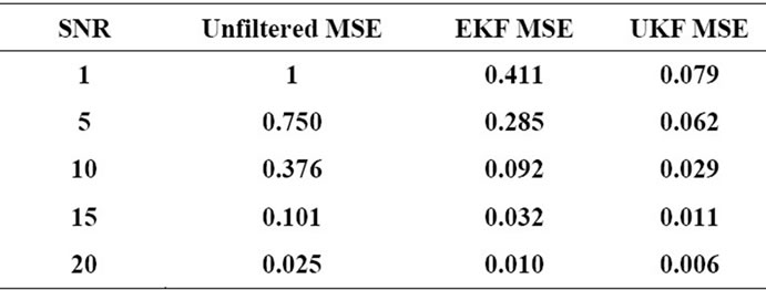
Table 1. Average MSEs of the unfiltered, EKF, and UKF estimated signals.
using a Bluetooth communication system model, which has been created in MATLAB/SIMULINK. Results have shown the effectiveness and superiority of UKF over EKF.
This method can be expanded to be implemented in other modulation schemes. There is more work that can be done to enhance the idea of this research by adding the fading processes to the channels. Also, the analysis of the Bluetooth system model can be expanded to include the effect of frequency hopping and interferences, and IKF can be modified to handle these disturbances. Also, more researches using different types of sigma-points methods can be conducted for more optimum results.
REFERENCES
- J. Proakis and M. Salehi, “Digital Communications,” 5th Edition, McGraw-Hill Higher Education, New York, 2008.
- M. Morelli, D. Benfatto, D. Lucano, M. Luise and U. Mengali, “Simple Non-Coherent Detectors for CPM Signals Transmitted over Rayleigh Flat-Fading Channels,” Proceedings of the 4th IEEE Workshop on Signal Processing Advances in Wireless Communications, Rome, 15-18 June 2003, pp. 492-496.
- W. P. Osborne and M. B. Luntz, “Coherent and Noncoherent Detection of CPFSK,” IEEE Transactions on Communications, Vol. 22, No. 8, 1974, pp. 1023-1036. doi:10.1109/TCOM.1974.1092333
- Bluetooth Special Interest Group (SIG), “Specification of the Bluetooth System, Core Version 4.0,” 2010. http://www.bluetooth.com
- A. G. Soltanian and R. E. Van Dyck, “Performance of the Bluetooth System in Fading Dispersive Channels and Interference,” Proceedings of the IEEE Global Telecommunications Conference, Vol. 6, 25-29 November 2001, pp. 3499-3503.
- T. Aulin and C.-E. Sundbergm, “Continuous Phase Modulation-Part I: Full Response Signaling,” IEEE Transactions on Communications, Vol. 29, No. 3, 1981, pp. 196-209. doi:10.1109/TCOM.1981.1095001
- L. Bin and P. Ho, “Data-Aided Linear Prediction Receiver for Coherent DPSK and CPM Transmitted over Rayleigh Flat-Fading Channels,” IEEE Transactions on Vehicular Technology, Vol. 48, No. 4, 1999, pp. 1229- 1236. doi:10.1109/25.775371
- J. Anderson, T. Aulin and C. Sundbergm, “Digital Phase Modulation,” Plenum Press, New York, 1986.
- N. Ibrahim, L. Lampe and R. Schober, “Bluetooth Receiver Design Based on Laurent’s Decomposition,” IEEE Transactions on Vehicular Technology, Vol. 56, No. 4, 2007, pp. 1856-1862. doi:10.1109/TVT.2007.897187
- M. Nafie, A. Gatherer and A. Dabak, “Decision Feedback Equalization for Bluetooth Systems,” Proceedings of the IEEE International Conference on Acoustics, Speech, and Signal Processing, Salt Lake City, May 2001, pp. 909- 912.
- H. Leib, “Data-Aided Noncoherent Demodulation of DPSK,” IEEE Transaction on Communications, Vol. 43, No. 234, 1995, pp. 722-725. doi:10.1109/26.380098.
- J. He, J. Cui, L. Yang and Z. Wang, “A Low-Complexity High-Performance Noncoherent Receiver for GFSK Signals,” Proceedings of the IEEE International Symposium on Circuits and Systems, Seattle, 18-21 May 2008, pp. 1256-1259.
- J. Gal, A. Campeanu and J. Nafornita, “Noncoherent Demodulation of Continuous Phase Modulated Signals Using Extended Kalman Filtering,” Proceedings of the IEEE 12th International Conference on Optimization of Electrical and Electronic Equipment, Basov, 20-22 May 2010, pp. 724-727.
- J. Gal, A. Campeanu and J. Nafornita, “Kalman Noncoherent Detection of CPFSK Signals,” Proceedings of the 8th International Conference Communications, Bucharest, 10-12 June 2010, pp. 65-68.
- O. Loffeld, “Demodulation of Noisy Phase or Frequency Modulated Signals with Kalman Filters,” Proceedings of the IEEE Acoustics, Speech, and Signal Processing, Adelaide, 19-22 April 1994, pp. IV/177-IV/180.
- R. E. Kalman, “A New Approach to Linear Filtering and Prediction Problems,” Research Institute for Advanced Study, Baltimore, 1960.
- M. S. Grewal and A. P. Andrews, “Kalman Filtering Theory and Practice Using MATLAB,” 3rd Edition, John Wiley & Sons, Inc, New York, 2008.
- J. Candy, “Bayesian Signal Processing Classical, Modern, and Particle Filtering Methods,” John Wiley & Sons, Inc, New York, 2009.
- D. Simon, “Optimal State Estimation, Kalman H∞, and Nonlinear Approaches,” John Wiley & Sons, Inc, New York, 2009.
- S. J. Julier and J. K. Uhlmann, “A New Extension of the Kalman Filter to Nonlinear Systems,” The 11th International Symposium of Aerospace/Defense Sensing, Simulation and Controls, Multi Sensor Fusion, Tracking and Resource Management II, Orlando, 20-25 April 1997, pp. 182-193.
- R. V. D. Merwe, “Sigma-Point Kalman Filters for Probabilistic Inference in Dynamic State-Space Models,” Ph.D. Thesis, OGI School of Science & Engineering at Oregon Health & Science University, 2004.
- S. J. Julier and J. K. Uhlmann, “Unscented Filtering and Nonlinear Estimation,” Proceedings of the IEEE, Vol. 92, No. 3, 2004, pp. 401-422. doi:10.1109/JPROC.2003.823141
- S. J. Julier, “The Scaled Unscented Transformation,” Proceedings of the 2002 American Control Conference, Vol. 6, 2002, pp. 4555-4559.
- S. J. Julier and J. K. Uhlmann, “Reduced Sigma Point Filters for the Propagation of Means and Covariances through Nonlinear Transformations,” Proceedings of the 2002 American Control Conference, Vol. 2, 2002, pp. 887-892.
- S. J. Julier and J. K. Uhlmann, “The Spherical Simplex Unscented Transformation,” Proceedings of the American Control Conference, Denver, 4-6 June 2003, pp. 2430- 2434. doi:10.1109/ACC.2003.1243439
- M. Ali and M. Zohdy, “Unscented Kalman Filtering for Continuous Phase Frequency Shift Keying Equalization”, Proceedings of the International Conference on Information and Industrial Electronics, Chengdu, 14-15 January 2011, pp. 20-25.
- T. S. Rappaport, “Wireless Communications Principles and Practice,”2nd Edition, Prentice Hall, Upper Saddle River, 2002.
- C. E. Sundberg, “Continuous Phase Modulation,” IEEE Communications Magazine, Vol. 24, No. 4, 1986, pp. 25- 38. doi:10.1109/MCOM.1986.1093063
- D. Labarre, E. Grivel, Y. Berthoumieu, E. Todini and M. Najim, “Consistent Estimation of Autoregressive Parameters from Noisy Observation Based on Two Interacting Kalman Filters,” Signal Processing, Vol. 86, No. 10, 2006, pp. 2863-2876.
- A. Jamoos, A. Abdo and H. Nour, “Estimation of OFDM Time-Varying Fading Channels Based on Two-CrossCoupled Kalman Filters,” Novel Algorithms and Technique in Telecommunications, Automation and Industrial Electronics, 2008, pp. 287-292. http://www.springerlink.com/content/978-1-4020-8736-3/#section=135616&page=1&locus=21
- E. Punskaya, C. Andrieu, A. Doucet and W. J. Fitzgerald, “Particle Filtering for Demodulation in Fading Channels with Non-Gaussian Additive Noise,” IEEE Transaction on Communications, Vol. 49, No. 4, 2001, pp. 579-582. doi:10.1109/26.917760
- L. Binh, “MATLAB Simulink Simulation Platform for Photonic Transmission Systems,” International Journal of Communications, Network and System Sciences, Vol. 2, 2009, pp. 91-168.