Open Journal of Modelling and Simulation
Vol.05 No.01(2017), Article ID:73746,32 pages
10.4236/ojmsi.2017.51009
Existence of Many Blue Shifted Galaxies in the Universe by Dynamic Universe Model Came True
Satyavarapu Naga Parameswara Gupta
Bhilai Steel Plant, Bhilai, India

Copyright © 2017 by author and Scientific Research Publishing Inc.
This work is licensed under the Creative Commons Attribution International License (CC BY 4.0).
http://creativecommons.org/licenses/by/4.0/


Received: March 17, 2016; Accepted: January 20, 2017; Published: January 23, 2017
ABSTRACT
There are many blue shifted Galaxies in our universe. Here we will see old simulations to make such predictions from the output graphs using SITA simulations. There are four new simulations also presented here. In these sets of simulations, different point masses are placed in different distances in a 3D Cartesian coordinate grid; and these point masses are allowed to move on universal gravitation force (UGF) acting on each mass at that instant of time at its position. The output pictures depict the three dimensional orbit formations of point masses after some iterations. In an orbit so formed, some Galaxies are coming near (Blue shifted) and some are going away (Red shifted). In this paper, the simulations predicted the existence of a large number of Blue shifted Galaxies, in an expanding universe, in 2004 itself. Over 8300 blue shifted galaxies have been discovered extending beyond the Local Group by Hubble Space Telescope (HST) in the year 2009. Thus Dynamic Universe model predictions came true.
Keywords:
Dynamic Universe Model, Blue Shifted Galaxies, Hubble Space Telescope (HST), SITA Simulations

1. Introduction
In this paper, the next part of this section gives a general introduction of Dynamic universe model. In the next section, we will discuss a brief history of Blue shifted Galaxies starting with Charles Messier. And in the third section we will go into prediction of Blue shifted Galaxies, how we will do and how the Red and Blue shifted Galaxies co-exist in this Universe. In further sub sections here we will discuss how Dynamic Universe Model tells about simultaneous existence of Blue and Red shifted Galaxies and the scenario of present-day peculiar motions of Galaxies, Hubble flow, Distant Red- shifted Galaxies. In the forth section we will discuss about the mathematics and initial values used for simulating the prediction process. In Section 5, we will discuss about graphs in the old and new SITA simulations used for prediction of Blue Shifted galaxies and all the resulting graphs and numerical outputs of four new simulations and the old simulations. The sixth is a discussion section, where we will see why the RATIO Blue to Red shifted galaxies will never be 50:50 and what are the other possible candidates for blue shifted galaxies. In section seven we will see the summary and conclusions.
Dynamic Universe model is a singularity free tensor based math model. The tensors used are linear without using any differential or integral equations. Only one calculated output set of values exists. Data means properties of each point mass like its three dimensional coordinates, velocities, accelerations and it’s mass. Newtonian two-body problem used differential equations. Einstein’s general relativity used tensors, which in turn unwrap into differential equations. Dynamic Universe Model uses tensors that give simple equations with interdependencies. Differential equations will not give unique solutions. Whereas Dynamic Universe Model gives a unique solution of positions, velocities and accelerations; for each point mass in the system for every instant of time. This new method of Mathematics in Dynamic Universe Model is different from all earlier methods of solving general N-body problem.
This universe exists now in the present state, it existed earlier, and it will continue to exist in future also in a similar way. All physical laws will work at any time and at any place. Evidences for the three dimensional rotations or the dynamism of the universe can be seen in the streaming motions of local group and local cluster. Here in this dynamic universe, both the red shifted and blue shifted Galaxies co-exist simultaneously.
In this paper, different sets of point masses were taken at different 3 dimensional positions at different distances. These masses were allowed to move according to the universal gravitation force (UGF) acting on each mass at that instant of time at its position. In other words each point mass is under the continuous and Dynamical influence of all the other masses. For any N-body problem calculations, the more accurate our input data the better will be the calculated results; one should take extreme care, while collecting the input data. One may think that “these are simulations of the Universe, taking 133 bodies is too less”. But all these masses are not same, some are star masses, some are Galaxy masses some clusters of Galaxies situated at their appropriate distances. All these positions are for their gravitational centres. The results of these simulation calculations are taken here.
Original submission of this paper “No Big bang and GR: proves DUMAS! (Dynamic Universe Model of cosmology: A computer Simulation)”, DSR894 was done on 2nd April 2004 to Physical Review D. Currently, this paper is being thoroughly revised and resubmitted. Here in these simulations the universe is assumed to be heterogeneous and anisotropic. From the output data graphs and pictures are formed from this Model. These pictures show from the random starting points to final stabilized orbits of the point masses involved. Because of this dynamism built in the model, the universe does not collapse into a lump (due to Newtonian gravitational static forces). This Model depicts the three dimensional orbit formations of involved masses or celestial bodies like in our present universe. From the resulting graphs one can see the orbit formations of the point masses, which were positioned randomly at the start. An orbit formation means that some Galaxies are coming near (Blue shifted) and some are going away (Red shifted) relative to an observer’s viewpoint.
New simulations were conducted. The resulting data graphs of these simulations with different kinds of input data are shown in this paper in the later parts.
In all these simulations, all point masses will have different distances, masses.
- Simulation 1: All point masses are Galaxies
- Simulation 2: All point masses are Globular Clusters
- Simulation 3: Globular Clusters 34 Galaxies 33 aggregates 33 conglomerations 33
- Simulation 4: Small star systems 10 Globular Clusters 100 Galaxies 8 aggregates 8 conglomerations 7
The problem with such simulations is the overwhelmingly large amounts of output data. Each simulation gives 3 dimensional vector data of accelerations, velocities, positions for every point mass in every iteration in addition to many types of derived data. A minimum of  dataset of 16 decimal digits will be generated in every iteration. It is data and data everywhere. It is a huge data mine indeed.
A point to be noted here is that the Dynamic Universe Model never reduces to General relativity on any condition. It uses a different type of mathematics based on Newtonian physics. This mathematics used here is simple and straightforward. As there are no differential equations present in Dynamic Universe Model, the set of equations give single solution in  Cartesian coordinates for every point mass for every time step. All the mathematics and the Excel based software details are explained in the three books published by the author [1] [2] [3] . In the first book, the solution to N-body problem-called Dynamic Universe Model (SITA) is presented; which is singularity-free, inter-body collision free and dynamically stable. The Basic Theory of Dynamic Universe Model published in 2010 [1] . The second book in the series describes the SITA software in EXCEL emphasizing the singularity free portions. This book written in 2011 [2] explains more than 21,000 different equations. The third book describes the SITA software in EXCEL in the accompanying CD/DVD emphasizing mainly HANDS ON usage of a simplified version in an easy way. The third book is a simplified version and contains explanation for 3000 equations instead of earlier 21,000 and this book also was written in 2011 [3] . Some of the other papers published by the author are available at Refs. [4] - [9] .
SITA solution can be used in many places like presently unsolved applications like Pioneer anomaly at the Solar system level, Missing mass due to Star circular velocities and Galaxy disk formation at Galaxy level etc. Here we are using it for prediction of blue shifted Galaxies.
2. History of Blue Shifted Galaxies―Let’s Start with Charles Messier
After 1922 Hubble published a series of papers in Astrophysical Journal describing various Galaxies and their red shifts/blue shifts. Using the new 100 inch Mt. Wilson telescope, Edwin Hubble was able to resolve the outer parts of some spiral nebulae as collections of individual stars and identified some Cepheid variables, thus allowing him to estimate the distance to the nebulae: they were far too distant to be part of the Milky Way. In the Ref. [10] [11] one can find more detailed analysis of this issue. And later using 200 inch Mt Palomar telescope Hubble could refine his search. In 1936 Hubble produced a classification system for galaxies that is used to this day, the Hubble sequence.
In the 1970s it was discovered in Vera Rubin’s study of the rotation speed of gas in galaxies that the total visible mass (from the stars and gas) does not properly account for the speed of the rotating gas. This galaxy rotation problem is thought to be explained by the presence of large quantities of unseen dark matter. This dark matter question was discussed by Vera Rubin, see the Ref. [12] [13] .
In fact there are millions of Blue shifted Galaxies not just 8300 found from 2009 by Hubble space telescope. ‘Beginning in the 1990s, the Hubble Space Telescope yielded improved observations. Among other things, Go to ADS search page try searching title and abstract with keywords “Blue shifted quasars”. If you search with “and” s i.e., ‘Blue and Shifted and Galaxies” [use “and” option not with “or” option] you will find 248 papers in ADS search. I did not go through all of them. it established that the missing dark matter in our galaxy cannot solely consist of inherently faint and small stars. One can find more detailed analysis of this issue in the published literature on Hubble Deep Field, They gave an extremely long exposure of a relatively empty part of the sky, provided evidence that there are about 125 billion (1.25 × 10¹¹) galaxies in the universe. Further details can be found at ref [10] . Improved technology in detecting the spectra invisible to humans (radio telescopes, infrared cameras, and x-ray telescopes) allow detection of other galaxies that are not detected by Hubble. Particularly, galaxy surveys in the Zone of Avoidance (the region of the sky blocked by the Milky Way) have revealed a number of new galaxies. In the Ref. [14] one can find more detailed analysis of this issue.
Hubble Space Telescope’s improved observational capabilities resolved as many as 8300 galaxies as Blue shifted till today which will discuss later in this paper, confirming that you have the correct template for your paper size. This template has been tailored for output on the custom paper size (21 cm × 28.5 cm).
3. Prediction of Blue Shifted Galaxies
3.1. Co-Existence of Red and Blue Shifted Galaxies
These simulations of Dynamic Universe Model predicted the existence of the large number of Blue shifted Galaxies in 2004, i.e., more than about 35 - 40 Blue shifted Galaxies known at the time of Astronomer Edwin Hubble in 1930s. See the ref [11] . The far greater numbers of Blue shifted galaxies was confirmed by the Hubble Space Telescope (HST) observations in the year 2009. Today the known number of Blue shifted Galaxies is more than 8300 scattered all over the sky and the number is increasing day by day. This is a greater number compared to 30 - 40 Blue shifted galaxies earlier.
In addition the author presumes that there is a greater probability that the Quasars, UV Galaxies, X-ray, γ-ray sources and other Blue Galaxies etc., are also Blue shifted Galaxies. Another assumption can be made about images of Galaxies. A safe assumption can be… out of a 930,000 Galaxy spectra in the SDSS database, about 40% are images for Galaxies; that leaves about 558,000 as Galaxies. If both the assumptions are correct, then there are 120,000 Quasars, 50,000 brotherhood of (X-ray, γ-ray, Blue Galaxies etc.,) of quasars, 8300 blue shifted galaxies. That is about 32% of available Galaxy count are Blue shifted. And if we don’t assume any images and assume about Quasars etc only, then it will be about 20% are Blue shifted Galaxies.
3.2. Dynamic Universe Model: Blue and Red Shifted Galaxies
In this Dynamic Universe Model―Galaxies in a cluster are rotating and revolving. Depending on the position of observer’s position relative to the set of galaxies, some may appear to move away, and others may appear to come near. The observer may also be residing in another solar system, revolving around the center of Milky Way in a local group. He is observing the galaxies outside. Many times he can observe only the coming near or going away component of the light ray called Hubble components. The other direction cosines of the movement may not be possible to measure exactly in many cases. It is an immensely complicated problem to untangle the two and pin point the cause of non-Hubble velocities. This question was discussed by J. V. Narlikar in (1983) see the ref [15] . “Nearby Galaxies Atlas” published by Tully and Fischer contains detailed maps and distribution of speeds of Galaxies in the relatively local region [16] . The multi component model used by them uses the method of least squares. Hence we can say that Galactic velocities are possible in all the directions Use a zero before decimal points: “0.25”, not “.25”. Use “cm3”, not “cc”.
3.3. Present-Day Peculiar Motions of Galaxies, Hubble Flow, Distant Red-Shifted Galaxies
“Peculiar motions” of Galaxies is the thing predicted by Dynamic Universe Model theoretically, whereas a Bigbang based cosmology predicts only radially outward motion from earth or red-shifted Galaxies and no blue-shifted Galaxies at all.
Local group of Galaxies are present up to a distance of 3.6 MPC. From that point onwards, we will find red-shifted Galaxies. I don’t know where actually Hubble flow starts. But I think that is the distance of 3.6 MPC where so called Hubble-flow starts. If the Hubble flow does not start here, why do red-shifted galaxies appear from this distance onwards? If the Hubble-flow is such strong, why would it leave some 8300 blue-shifted Galaxies? Anybody can see the updated list of Blue shifted Galaxies in the NED. (NASA/IPAC EXTRAGALACTIC DATABASE) by JPL anybody can get the exact number of Blue shifted Galaxies by Hubble space telescope to the present date & time. (If you need any assistance in searching NED, please contact the author) As on 4th April 2012 at 1210 hrs Indian time, it is 7306 Blue-shifted galaxies. But presently this search gives 8300. Some current active research and discussions can be found in physics forums by searching “blue-shifted-galaxies-there-are-more”.
We are discussing “Hubble flow” as some unknown force pulling away all the galaxies to cause the expansion of universe. But in reality it is the going away component of “peculiar motion” of that particular Galaxy. That Galaxy may be moving in any direction in reality. Each Galaxy move independently, with the gravitational force of its Local group, clusters etc. There is no separate Hubble force to cause a separate Hubble flow …
Different estimates of distances of Blue-shifted Galaxies especially in Virgo Cluster are varying. There are about 3000 blue-shifted Galaxies in Virgo cluster. Some estimate for the most distant Blue-shifted Galaxy in Virgo cluster may go as high as 40 MPC, and other estimate go as low as 17 MPC. I don’t know whom to believe. Here distance estimate is not dependent on Red/Blue shift, but dependent on various other methods. Here probably the distance and red shift proportionality is not working. So we can see that blue shifted Galaxies are not confining to earlier thinking of 3.6 MPC distances. Here, the estimated distance is not depending on Red/Blue shift, but on various other methods. Accurate measurement of distances after 40 MPC depends mostly on red- shift only. There is a hope to find an accurate estimate of distance, if type 1a Supernova standard candle is observed in a Galaxy. When we are estimating the distance with red-shift, finding far off blue-shifted Galaxies is not possible.
All these findings are from some recent times only. Hence nothing can be said about the peculiar motions of blue shifted Galaxies. All these velocities are at present radial velocities only. A lot of work is to be done in these lines.
In general, whether the Source is emitting radiation in Infrared (Microwave or some lover frequencies) region or lower, or the Source is in Ultra violet (X-rays or higher) frequency region, we take the source as red-shifted only. The sources which emit only X-rays were taken as red-shifted, though by definition, X-rays are blue-shifted, due to their higher frequency. Even if the source is emitting a single frequency radiation, we find it is only red-shifted.
4. Using the Template
Let us assume heterogeneous and anisotropic set of N particles/point masses moving under mutual gravitation as a system, and these particles/point masses are also under the gravitational influence of other systems with a different number of particles/point masses in different systems. For a broader perspective, let us call this set of all the systems of particles/point masses as an Ensemble. Let us further assume that there are many Ensembles each consisting of a different number of systems with different number of particles/point masses. Similarly, let us further call a group of Ensembles as Aggregate. Let us further define a Conglomeration as a set of Aggregates and let a further higher system have a number of conglomerations and so on and so forth.
Now for the start, let us assume a set of N mutually gravitating particles/point masses in a system. Let the  particle/point mass has mass
 , and is in position
 . In addition to the mutual gravitational force, there exists an external
 , due to other systems, ensembles, aggregates, and conglomerations etc., which also influence the total force
  acting on the particle
 . Here in this case, the
  is not a constant universal Gravitational field but it is the total vectorial sum of fields at
  due to all the particles/point masses external to its system bodies and with that configuration at that moment of time, external to its system of N particles/point masses.
 (1)
(1)
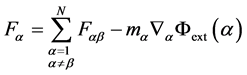
Total force on the particle  is
is , Let
, Let  is the gravitational force on the
  th particle/point mass due to
  particle.
 (2)
(2)
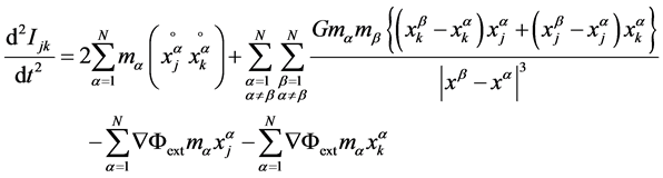
Moment of inertia tensor
Consider a system of N particles/point masses with mass , at positions
 ; The moment of inertia tensor is in external back ground field
 .
.
 (3)
(3)
Its second derivative is [Equation (4) removed]
 (5)
(5)
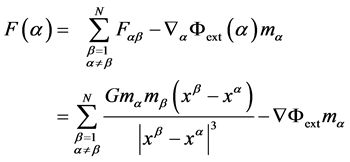
The total force acting on the particle  is and
  is the unit vector of force at that place of that component.
 (6)
(6)
Writing a similar formula for 
 (7)
(7)
or
 (8)
(8)
and
 (8a)
(8a)
Lets define Energy tensor ( in the external field )
)
 (9)
(9)
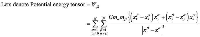 (10)
(10)
 (11)
(11)
 (12)
(12)
Hence
 (13)
(13)
Here in this case
 (14)
(14)
 (15)
(15)
 (16)
(16)
We know that the total force at 
 (17)
(17)
There fore total Gravitational potential  (α) at
  per unit mass
 (18-s)
Lets discuss the properties of :-
:-
 can be subdivided into 3 parts mainly
 due to higher level system,
  due to lower level system,
  due to present level. [Level: when we are considering particles in the same system (Galaxy) it is same level, higher level is cluster of galaxies, and lower level is planets & asteroids].
 due to lower levels : If the lower level is existing, at the lower level of the system under consideration, then its own level was considered by system equations. If this lower level exists anywhere outside of the system, centre of (mass) gravity outside systems (Galaxies) will act as unit its own internal lower level practically will be considered into calculations. Hence consideration of any lower level is not necessary.
SYSTEM―ENSEMBLE:
Until now we have considered the system level equations and the meaning of . Now let’s consider an ENSEMBLE of system consisting of
  particles in each. These systems are moving in the ensemble due to mutual gravitation between them. For example, each system is a Galaxy, and then ensemble represents a local group. Then number of Galaxies is
 , Galaxies are systems with particles
 , we will consider
  as discussed above. That is we will consider the effect of only higher level like external Galaxies as a whole, or external local groups as a whole.
Ensemble Equations (Ensemble consists of many systems)
 (18-E)
Here  denotes Ensemble.
This  is the external field produced at system level. And for system
 (13)
(13)
Assume ensemble in a isolated place. Gravitational potential  produced at system level is produced by Ensemble and
  as ensemble is in an isolated place.
 (19)
(19)
There fore
 (20)
(20)
and
 (21)
(21)
AGGREGATE Equations (Aggregate consists of many Ensembles)
 (18-A)
Here  denotes Aggregate.
This  is the external field produced at Ensemble level. And for Ensemble
 (18-E)
Assume Aggregate in an isolated place. Gravitational potential  produced at Ensemble level is produced by Aggregate and
  as Aggregate is in a isolated place.
 (22)
(22)
Therefore
 (23)
(23)
And
 (24)
(24)
Total AGGREGATE Equations: (Aggregate consists of many Ensembles and systems)
Assuming these forces are conservative, we can find the resultant force by adding separate forces vectorially from Equations ((20) and (23)).
 (25)
(25)
This concept can be extended to still higher levels in a similar way.
Corollary 1:
 (13)
(13)
The above equation becomes scalar Virial theorem in the absence of external field, that is  and in steady state,
i.e. (27)
(27)
 (28)
(28)
But when the N-bodies are moving under the influence of mutual gravitation without external field then only the above Equation (28) is applicable.
Corollary 2:
Ensemble achieved a steady state,
i.e. (29)
(29)
 (30)
(30)
This  external field produced at system level. Ensemble achieved a steady state; means system also reached steady state.
i.e. (27)
(27)
 (31)
(31)
Combining both 3 and 25 (Newly introduced in this paper)
 (32)
(32)
So…
 (33)
(33)
Interchanging  and
and  operations:
 (34)
(34)
or
 (35)
(35)
The above Equation (35) means the force on  point mass will be a sum of three components i.e., the summation of attraction forces due to point masses from its own system, ensemble and aggregate. This is the key result that can be applied to point masses or subatomic particles or combined in any fashion together. The Equations ((34) & (35)) are important, simple & straight forward results.
Table of Initial Values for New Blue Shifted Galaxies Simulation
Any simulation requires initial data, and the initial data for one of these simulations is shown here. Table 1 describes the simulated initial values used in one of the new SITA calculations. In this particular simulation Globular clusters (system * 109) are 34 numbers, galaxies (Ensemble) are 33, clusters of Galaxies (aggregates) are 33 and groups of Galaxy clusters (Conglomeration) are 33. Data for other simulations can be received from me. This table is shown in Appendix 1.
This Table 1 describes the simulated initial values used in SITA calculations. In this simulation Globular clusters (system * 109) are 34 no’s, galaxies (Ensemble) are 33, clusters of Galaxies (aggregates) are 33 no’s, Groups of Galaxy clusters (Conglomeration) are 33 nos. The name field gives list of various point masses. Columns heads have names “Mass simu (kg), xsimu (M), ysimu (M) and zsimu (M)”, the column “Masssimu (kg)” contains simulated values for Mass in Kg and columns “xsimu (M), ysimu (M) and zsimu (M)” contain  and
and  Cartesian coordinates in meters.
5. SITA: Blue Shifted Galaxies Graphs and Numerical Outputs & New Simulations
Resulting graphs of old simulations for Blue Shifted Galaxies
Positioning From these resulting graphs one can see the orbit formations. When a uniform density of matter is assumed, say an equal point mass is placed in a uniform way in a three dimensional grid, all the point masses are collapsing into the CG of the set of masses. That means all are coming near and are Blue shifted. Orbit formations are happening only in non-uniform density distributions.
All the calculations were done using a small number of point masses. But the results were extremely encouraging. Always similar mass structures at large scale were formed in three dimensions showing lumpy formulations. Higher (super) computers can take up more number of point masses and show the empty nature of the formation to a greater detail in a faster manner.
Irrespective various starting positions of masses, the final stabilized mass positions are similar. The higher distance between the masses like great walls, the faster the movements are. The extremely distant galaxies are moving faster with huge red and blue shirts and with high velocities. The fallowing graphs are from the old 2004 paper. In this paper only typical pictures were presented. These figures are shown in Appendix 2.
There is no gravitational collapse of masses. Here there was no gravitational repulsion was present. All masses form orbits and move in orbits.
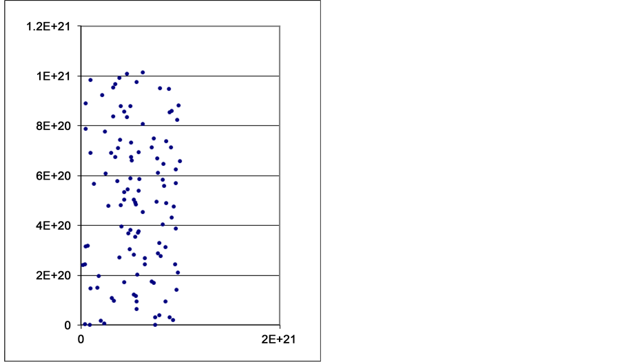
Graph G1: starting pictures of  positions of Clusters (right) and Globular Clusters (left),
  and
and  axes scales represent distances in meters. These masses are randomly on
  axes. An orbit formation means some Galaxies are coming near (Blue shifted) and some are going away (Red shifted).
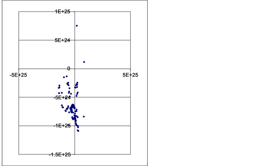
Graph G2 and Graph G3 represent the positions of all masses in this simulation, after one time-step and two time-steps. Here the masses hidden in the Graph G1 are also visible which were visible as a small dot near the zero of  axes, and which were shown in Graph G1 in a more elaborate way. We can see the formation of some three- dimensional circles clearly.
Graph G4 represents the positions of all masses in this simulation, after three and four time-steps. We can see the formation of some three-dimensional circles clearly.
Graph G5 represents the positions of all masses in this simulation, after four time-steps and seven time-steps. We can see the formation of some three-dimensional circles clearly. That means orbit formation.
5.1. Four New Simulations
New simulations were carried out on this subject. These are four more simulations with different kinds of input data. Four more files are being attached in Excel format which have all the output 3000 graphs and initial input data. Each is about 10 MB. In all these four simulations, all point masses have different distances and masses. The simulations are:
- All point masses are Galaxies
- All point masses are Globular Clusters
- Globular Clusters 34 Galaxies 33 aggregates 33 conglomerations 33
- Small star systems 10 Globular Clusters 100 Galaxies 8 aggregates 8 conglomerations 7
Rotations of Galaxies and orbit formations are visible in all types of formations. I will send any other data files upon further request.
5.2. Results of New Simulations
Rotations of Galaxies and orbit formations are visible in all types of formations.
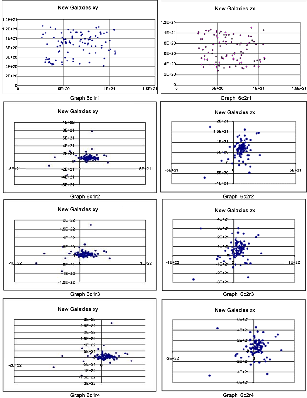
5.3. Graphs from “All Point Masses are Clusters (Approximately 109 Stars)” Simulation
These graphs are shown in Appendix 3
In the above set of figures First column group of Graphs were with the name New Galaxies . Figures in the second column group of Graphs were with the name ‘New all zx’p”. These are
  and
and  plots of positions of Clusters approximately have the mass of about a billion or 109 solar masses. First set is about 100 and second set is for all 133 Galaxies/clusters. All these are point masses for Galaxies but of smaller sizes. The word ‘new’ in the name is an indicative word for the result of that particular iteration in the simulation. The first iteration is the starting positions of the Galaxies in
  or
or  plots. From that with a time step of 3.15576E+15 seconds or 100 million years is allowed for the free fall of all the Galaxies. Next set of positions is shown in the iteration 1. After that is iteration 2 and so on. One can see the rotations of these masses. And the marked change of positions from iteration to iteration when we look through the series of graphs.
Graphs 3c1r1, 3c2r1 show the initial random positions in ‘ ’ and ‘
 ’ views in Cartesian coordinates for the simulation “all point masses are Clusters (approximately 109 stars)”.
Graphs 3c1r2, 3c2r2 show the positions after few iterations in ‘ ’ and ‘
 ’ views in Cartesian coordinates, one can see disk formation and none of the point masses collapse into lump due to mutual gravitation.
Graphs 3c1r3, 3c2r3 show the positions after additional few iterations as shown in 3c1r2, 3c2r2 graphs. Here one can see similar disk formed earlier but AGAIN in different size and shape due to combined effect of mutual gravitation and acquired velocities called Universal Gravitation Force (UGF) acting on each point mass.
Hence one can see all the Galaxies are moving due to UGF and orbit formations are there. That means these Galaxies have peculiar motions and some Galaxies appear to be moving away and some other Galaxies are coming near. Hence Blue shifted Galaxies exists
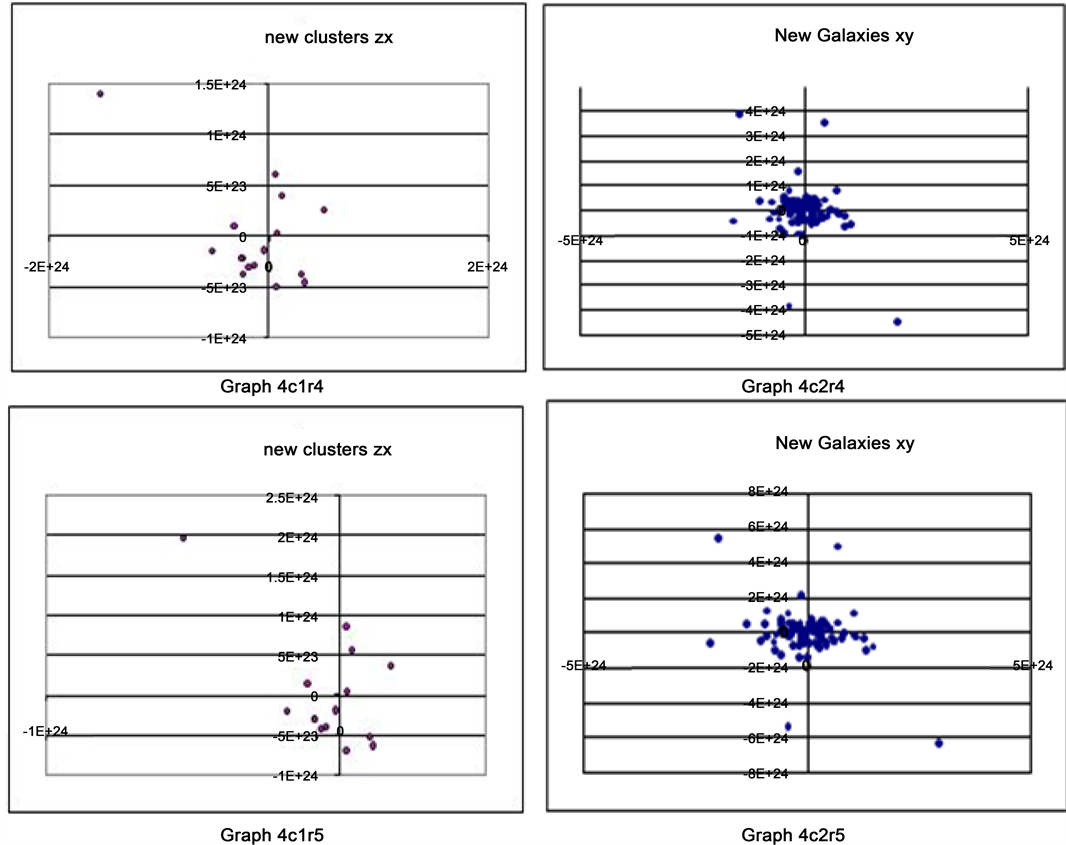
5.4. Graphs from “All Point Masses are Galaxy Ensembles” Simulation
These graphs are shown in Appendix 4.
Here in this example (in this new simulation), in the above set of figures, the first column group of Graphs were with the name New Clusters . Figures in the second column group of Graphs were with the name New Galaxies
 . These are
  and
and  plots of positions of Clusters (or Galaxies) approximately have the mass of about a billion or 1012 solar masses. First set is about 20 and second set is for all 100 Galaxies/clusters. All these are point masses for Galaxies of normal sizes. The word “new” in the name is an indicative word for the result of that particular iteration in the simulation. The first iteration is the starting positions of the Galaxies in
  or
or  plots. From that with a time step of 3.15576E+15 seconds or 100 million years is allowed for the free fall of all the Galaxies. Next set of positions is shown in the iteration 1. After that is iteration 2 and so on. One can see the rotations of these masses. And the marked change of positions from iteration to iteration when we look through the series of graphs.
The set of graphs depicting the positions of all the point masses were omitted here due to space constraints. The change in positions is visible only in the first few graphs for all the point mass positions.
The “New clusters ” graphs indicate a subset of all Galaxies is rotating about. These graphs will show the observer, some Galaxies are coming near and some are going away. Hence these galaxies are either red shifted or blue shifted.
Graphs 4c1r1, 4c2r1 show the initial random positions in “ ” and “
 ” views in Cartesian coordinates for the simulation “All point masses are Galaxy Ensembles’ simulation”.
Graphs 4c1r2, 4c2r2 show the positions after few iterations in “ ” and “
 ” views in Cartesian coordinates, one can see disk formation and none of the point masses collapse into lump due to mutual gravitation.
Graphs 4c1r3, 4c2r3 to 4c1r4, 4c2r4 show the positions after additional few iterations as shown in 4c1r2, 4c2r2 graphs. Here one can see similar disk formed earlier but AGAIN in different size and shape due to combined effect of mutual gravitation and acquired velocities called Universal Gravitation Force (UGF) acting on each point mass.
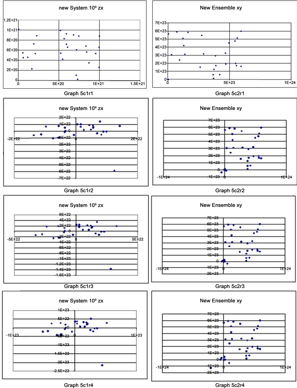
5.5. Graphs from “Globular Clusters 34 Galaxies 33 Aggregates 33 Conglomerations 33” Simulation
These graphs are shown in Appendix 5.
Here in this example (in this new simulation), in the above set of figures, the first column group of Graphs were with the name New System 109 . Figures in the second column group of Graphs were with the name New Ensembles
 . These are
  and
and  plots of positions of Globular Clusters and Galaxies approximately have the mass of about 100 million to a billion or 1012 solar masses. First set is about 34 and second set is for all 33 Galaxies. All these are point masses for Galaxies of normal sizes. The word “new” in the name is an indicative word for the result of that particular iteration in the simulation. The first iteration is the starting positions of the Galaxies in
  or
or  plots. From that with a time step of 3.15576E+16 seconds or one billion years is allowed for the free fall of all the Galaxies. Next set of positions is shown in the iteration 1. After that is iteration 2 and so on. One can see the rotations of these masses. And the marked change of positions from iteration to iteration when we look through the series of graphs.
The set of graphs depicting the positions of all the point masses were omitted here due to space constraints. The change in positions is visible only in the first few graphs for all the point mass position graphs.
These two columns of graphs indicate all Galaxies are rotating about. These graphs show to the observer, some Galaxies are coming near and some are going away. Hence these galaxies are either red shifted or blue shifted.
Graphs 5c1r1, 5c2r1 show the initial random positions in “ ” and “
 ” views in Cartesian coordinates for the simulation “All point masses are Galaxy Ensembles’ simulation”.
Graphs 5c1r2, 5c2r2 show the positions after few iterations in “ ” and “
 ” views in Cartesian coordinates, one can see disk formation and none of the point masses collapse into lump due to mutual gravitation.
Graphs 5c1r3, 5c2r3 to 5c1r8, 5c2r8 show the positions after additional few iterations as shown in 4c1r2, 4c2r2 graphs. Here one can see similar disk formed earlier but AGAIN in different size and shape due to combined effect of mutual gravitation and acquired velocities called Universal Gravitation Force (UGF) acting on each point mass.
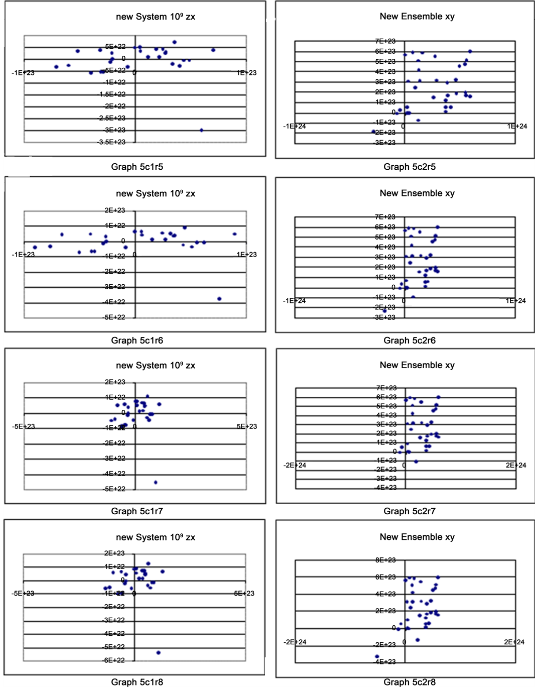
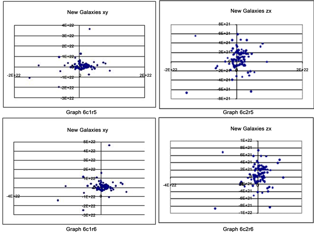
5.6. Graphs from “Small Star Systems 10 Globular Clusters 100 Galaxies 8 Aggregates 8 Conglomerations 7” Simulation
These graphs are shown in Appendix 6.
Here in this fourth example (in this new simulation), in the above set of figures, the first column group of Graphs were with the name New Galaxies . Figures in the second column group of Graphs were with the name New Galaxies
 . These are
  and
and  plots of positions of 100 Galaxies approximately have the mass of about a billion or 1012 solar masses.
Here  and
and  plots of the same 3 dimensional point mass positions were chosen so that one can imagine the three dimensional picture of the same set. These graphs represent the output of SITA simulations for the same iteration and for the same set of masses.
All these are point masses for Galaxies of
normal sizes. The word “new” in the name is an indicative word for the result of that particular iteration in the simulation. The first iteration is the starting positions of the Galaxies in  or
or  plots. From that with a time step of 3.15576E+15 seconds or one billion years is allowed for the free fall of all the Galaxies. Next set of positions is shown in the iteration 1. After that is iteration 2 and so on. One can see the rotations of these masses. And the marked change of positions from iteration to iteration when we look through the series of graphs.
The set of graphs depicting the positions of all the point masses, all other different varieties of masses were omitted here due to space constraints. The change in positions is visible only in the first few graphs for all the point mass position graphs.
These two columns of graphs indicate that all Galaxies are rotating about. These graphs show to the observer, some Galaxies are coming near and some are going away. Hence these galaxies are either red shifted or blue shifted.
Graphs 6c1r1, 6c2r1 show the initial random positions in ‘ ’ and ‘
 ’ views in Cartesian coordinates for the simulation “All point masses are Galaxy Ensembles’ simulation”.
Graphs 6c1r2, 6c2r2 show the positions after few iterations in ‘ ’ and ‘
 ’ views in Cartesian coordinates, one can see disk formation and none of the point masses collapse into lump due to mutual gravitation.
Graphs 6c1r3, 6c2r3 to 6c1r6, 6c2r6 show the positions after additional few iterations as shown in 6c1r2, 6c2r2 graphs. Here one can see similar disk formed earlier but AGAIN in different size and shape due to combined effect of mutual gravitation and acquired velocities called Universal Gravitation Force (UGF) acting on each point mass.
6. Discussion
In this model both red shift and blue shift of galaxies are possible simultaneously in all directions and at all distances from us. That depends only on location of distant rotating and revolving cluster.
We can say that:
1) The RATIO Blue to Red shifted galaxies will never be 50:50
2) The galaxies that appear to come near (Blue Shifted) will always present in the total number of galaxies. This number is not zero as predicted by expanding universe models.
3) The percentage of blue shifted galaxies will vary from place to place. That depends on many factors, like the FORMATION OF IMAGES IN THAT AREA. Images may be formed for the whole of local group itself.
4) The number of blue shifted Galaxies depend on the orientation of the planar revolving cluster of galaxies with respect us.
5) We will assume Hubble law for empirical distances of galaxies as . Where v is the velocity of the galaxy, c is the velocity of light, z is the red shift, D is the distance of galaxy,
  is the Hubble constant for distance only not for expansion of universe.
The galaxies that appear to come near (Blue Shifted) will always present in the total number of galaxies. This number is not zero as predicted by expanding universe models. The percentage of blue shifted galaxies will vary from place to place. That depends on many factors, like the formation of images in that area. Images may be formed for the whole of local group itself. The number of blue shifted Galaxies depends on the orientation of the plane of revolving cluster of galaxies with respect us. For obtaining the real map of Universe, we have to eliminate all the images from the Map, for which a detailed probing of all Galaxies is required.
6.1. Types of Blue Galaxies Whose Radiation Is Found in UV and Above Frequencies (Blue Shifted Galaxies)
There are many types of Galaxies. Many of them are into blue shift. Some types like Starburst, AGNs, UV and Gamma ray can be a safe bet for blue shifted Galaxy candidates. Classifying the starburst/AGN category itself isn’t easy since starburst galaxies don’t represent a specific type in themselves. Blue shifted Galaxies can occur in disk galaxies, spherical in any other shapes. And especially in irregular galaxies which often exhibit knots of starburst, often spread throughout the irregular galaxy are possible Blue shifted Galaxies. Let’s see various possible Blue shifted Galaxies below:
Blue compact galaxies (BCGs), Active galactic nucleus (AGN), Radio-quiet AGN, Seyfert galaxies, Radio-quiet quasars/QSOs, “Quasar 2s”, Radio-loud quasars, Radio-quit quasars, “Blazars” (BL Lac objects and OVV quasars), Radio galaxies, Blue compact dwarf galaxies(BCD galaxy), Pea galaxy (Pea galaxies), Luminous infrared galaxies (LIRGs), Ultra-luminous Infrared Galaxies (ULIRGs), and Hyperluminous Infrared galaxies (HLIRGs).
6.2. Evidences for AGNs and Quasars are Blue Shifted Galaxies― Present Day Concept of Quasars
Quasars are among the most luminous, powerful and energetic objects known in the universe and can emit up to a thousand times the energy output of the Milky Way [13] . Quasars have all the same properties as active galaxies and AGNs, but are more powerful. The radiation emitted by quasars is across the spectrum, almost equally, from X-rays to the far-infrared with a peak in the ultraviolet-optical bands, with some quasars also being strong sources of radio emission and of gamma-rays. Additionally Quasars can be detected over the entire observable electromagnetic spectrum including radio, infrared, optical, ultraviolet, X-ray and even gamma rays. Their radiation is partially “non-thermal” i.e., not due to a black body. In early optical images, quasars looked like single points of light (i.e., point sources), indistinguishable from stars, except for their peculiar spectra. With infrared telescopes and the Hubble Space Telescope, the “host galaxies” surrounding the quasars have been identified in some cases. These galaxies are normally too dim to be seen against the glare of the quasar, except with these special techniques. Most quasars cannot be seen with small telescopes, but 3C 273, with an average apparent magnitude of 12.9, is an exception. At a distance of 2.44 billion light- years, it is one of the most distant objects directly observable with amateur equipment. In Part 4, this quasar 3C 273 was shown to have a blue shift of (0.143122).
About 8% to 15% of Quasars have jets with lengths of millions of light years. These jets carry significant amounts of energy in the form of high-energy particle that move with speeds close to the speed of light consisting of either electrons and protons or electrons and positrons.
The Active Galactic Nuclei popularly known as AGNs and Quasars are Blue shifted Galaxies. Let us discuss about the quasars and AGNs in a next paper. One can see [16] [17] [18] [19] for additional information.
7. Conclusions
Hence we may conclude:
The actual ratio of Red shifted to Blue shifted Galaxies will depend on
a) Universal Gravitational Force acting on each Galaxy at that instant of time,
b) The position of the observer in the Universe,
c) The actual point mass distribution in the universe in three dimensions at that instant of time. This ratio can never be 50:50.
Dynamic Universe model is based on hard observed facts and gives many verifiable facts. In this paper the simulations predicted the existence of the large number of Blue shifted Galaxies, in an expanding universe, in 2004 itself. It was confirmed by Hubble Space Telescope (HST) observations in the year 2009. This prediction process is clearly shown the output pictures formed from this Model from old and new simulations. These pictures depict the three dimensional orbit formations. An orbit formation means some Galaxies are coming near (Blue shifted) and some are going away (Red shifted). This paper goes on two main lines. First is the main line of thinking, to show mathematically that there will be lots and lots of blue shifted Galaxies. To support this concept the question what are the possible blue shifted Galaxies is answered further. We find that quasars are blue shifted galaxies. The second line of thinking goes with this finding, that the Quasars are blue shifted galaxies. Now it can be 32% of total Galaxies are blue shifted in this universe.
Acknowledgements
I sincerely thank Maa Vak for continuously guiding this research. For helpful editing remarks I sincerely thank Dr. Lukasz Andrzej Glinka of Poland.
Cite this paper
Gupta, S.N.P. (2017) Existence of Many Blue Shifted Galaxies in the Universe by Dynamic Universe Model Came True. Open Journal of Modelling and Simulation, 5, 113-144. http://dx.doi.org/10.4236/ojmsi.2017.51009
References
- 1. Gupta, S.N.P. (2010) Dynamic Universe Model: A Singularity-Free N-Body Problem Solution. VDM Publications, Saarbrucken.
http://vaksdynamicuniversemodel.blogspot.in/p/books-published.html - 2. Gupta, S.N.P. (2011) Dynamic Universe Model: SITA Singularity Free Software. VDM Publications, Saarbrucken.
http://vaksdynamicuniversemodel.blogspot.in/p/books-published.html - 3. Gupta, S.N.P. (2011) Dynamic Universe Model: SITA Software Simplified. VDM Publications, Saarbrucken.
http://vaksdynamicuniversemodel.blogspot.in/p/books-published.html - 4. Gupta, S.N.P., Murty, J.V.S. and Krishna, S.S.V. (2014) Mathematics of Dynamic Universe Model Explain Pioneer Anomaly. Nonlinear Studies USA, 21, 26-42.
- 5. Gupta, S.N.P. (2013) Introduction to Dynamic Universe Model. International Journal of Scientific Research and Reviews Journal, 2, 203-226.
- 6. Gupta, S.N.P. (2015) “No Dark Matter” Prediction from Dynamic Universe Model Came True! Journal of Astrophysics and Aerospace Technology, 3, 1000117.
- 7. Gupta, S.N.P. (2014) Dynamic Universe Model’s Prediction “No Dark Matter” in the Universe Came True! Applied Physics Research, 6, 8-25.
- 8. Gupta, S.N.P. (2015) Dynamic Universe Model Predicts the Live Trajectory of New Horizons Satellite Going to Pluto. Applied Physics Research, 7, 63-77.
- 9. Gupta, S.N.P. (2014) Dynamic Universe Model Explains the Variations of Gravitational Deflection Observations of Very-Long-Baseline Interferometry. Applied Physics Research, 6, 1-16.
- 10. Tipler, F.J. (1996) Newtonian Cosmology Revisited. Monthly Notices of Royal Astronomical Society, 282, 206-210.
https://doi.org/10.1093/mnras/282.1.206 - 11. Shi, X. and Turner, M.S. (1998) Expectations for the Difference between Local and Global Measurements of the Hubble Constant. Astrophysics Journal, 493, 519-522.
https://doi.org/10.1086/305169 - 12. Rubin, V.C. (1983) Dark Matter in Spiral Galaxies. Scientific American, 248, 96-106.
https://doi.org/10.1038/scientificamerican0683-96 - 13. Rubin, V.C. (2000) One Hundred Years of Rotating Galaxies. Publications of the Astronomical Society of the Pacific, 112, 747-750.
https://doi.org/10.1086/316573 - 14. Aguirre, A. and Gratton, S. (2002) Steady-State Eternal Inflation. Physical Review D, 65, Article ID: 083507.
https://doi.org/10.1103/PhysRevD.65.083507 - 15. Narlikar, J.V. (1983) Introduction to Cosmology. Foundation Books, New Delhi.
- 16. Tully, R.B. and Fisher, J.R. (1987) Nearby Galaxies Atlas. Cambridge University Press, Cambridge, England.
- 17. Einstein, A. (1952) The Foundation of the General Theory of Relativity. In: Lorentz, H.A., Einstein, A., Minkowski, H. and Weyl, H., Eds., The Principle of Relativity: A Collecton of Original Memoirs on the Special and General Theory of Relativity, with Notes by A. Sommerfeld, Dover, USA, 109-164.
- 18. Obukhov, Y.N. (1992) Rotation in Cosmology. General Relativity and Gravitation, 24, 121-128.
https://doi.org/10.1007/BF00756780 - 19. Carneiro, S. (2000) A Gödel-Friedmann Cosmology? Physical Review D, 61, Article ID: 083506.
https://doi.org/10.1103/PhysRevD.61.083506
Appendix 1
Initial values Table for simulation “Globular Clusters 34 Galaxies 33 aggregates 33 conglomerations 33”

Table 1. Describes the simulated initial values used in SITA calculations. In this simulation Globular clusters (system * 109) are 34 no’s, galaxies (Ensemble) are 33, clusters of Galaxies (aggregates) are 33 no’s, Groups of Galaxy clusters (Conglomeration) are 33 nos. The name field gives list of various point masses. Columns heads have names “Mass simu(kg), xsimu (M), ysimu (M) and zsimu (M)”, The column “Masssimu(kg)” contains simulated values for Mass in Kg and columns “xsimu (M), ysimu (M) and zsimu (M)” contain x, y and z Cartesian coordinates in meters.
Appendix 2
The following graphs are from the old 2004 paper. In this paper only typical pictures were presented.
Graph G1. Initial random positions.

Graph G2. Picture after one time step, a lump formation was seen.
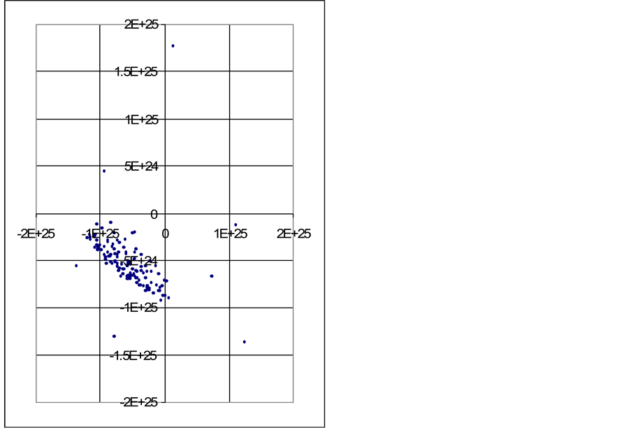
Graph G3. Now after two time steps the lump was stretched. Lump was still stretched after 3 time steps and initial mass rotation formations are seen.

Graph G4. Randomly positioned masses started showing circular orbit formations.
Graph G5. Orbit formations are clearer and all masses started following huge orbits depending on the masses.
Appendix 3
Graphs from “all point masses are Clusters (approximately 109 stars)” simulation
Appendix 4
Graphs from “All point masses are Galaxy Ensembles” simulation
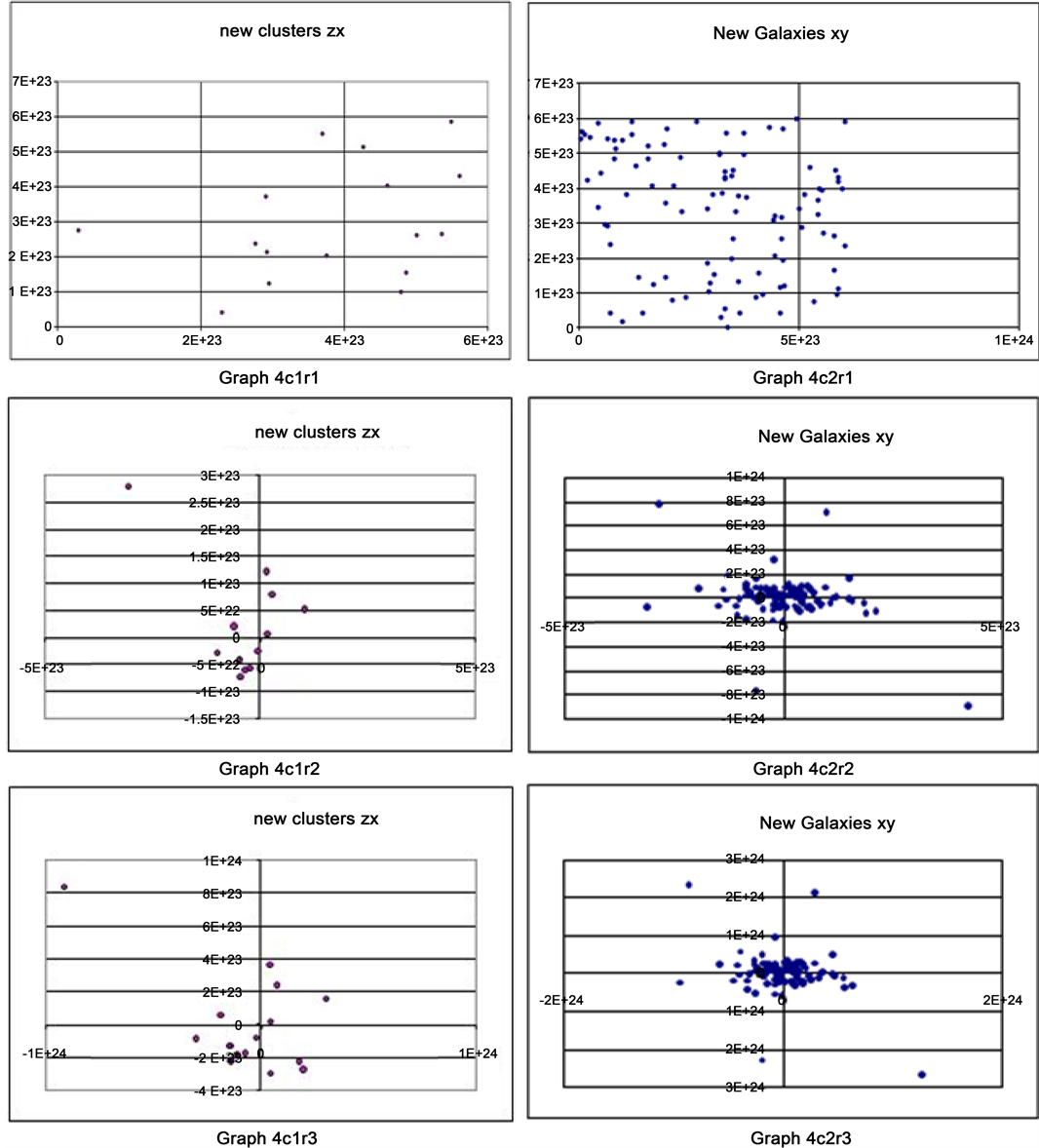
Appendix 5
Graphs from “Globular Clusters 34 Galaxies 33 aggregates 33 conglomerations 33” simulation
Appendix 6
Graphs from ‘Small star systems 10 Globular Clusters 100 Galaxies 8 aggregates 8 conglomerations 7’ simulation

Submit or recommend next manuscript to SCIRP and we will provide best service for you:
Accepting pre-submission inquiries through Email, Facebook, LinkedIn, Twitter, etc.
A wide selection of journals (inclusive of 9 subjects, more than 200 journals)
Providing 24-hour high-quality service
User-friendly online submission system
Fair and swift peer-review system
Efficient typesetting and proofreading procedure
Display of the result of downloads and visits, as well as the number of cited articles
Maximum dissemination of your research work
Submit your manuscript at: http://papersubmission.scirp.org/
Or contact ojmsi@scirp.org