International Journal of Geosciences
Vol.07 No.03(2016), Article ID:65016,8 pages
10.4236/ijg.2016.73027
Anisotropy and Empirical Relations for the Estimation of Anisotropy Parameters in Niger Delta Depobelts
Iheanyichukwu P. C. Okorie*, Joseph O. Ebeniro, Chukwuemeka N. Ehirim
Geophysics Research Group, Physics Department, University of Port Harcourt, Port Harcourt, Nigeria

Copyright © 2016 by authors and Scientific Research Publishing Inc.
This work is licensed under the Creative Commons Attribution International License (CC BY).
http://creativecommons.org/licenses/by/4.0/


Received 27 November 2015; accepted 22 March 2016; published 25 March 2016
ABSTRACT
The difficulty in achieving well-to-seismic ties due to errors arising from wrong time-to-depth conversions has been as a result of ignoring anisotropy in seismic processing. Anisotropy plays a vital role in the processing and interpretation of seismic data. In this work, an inversion method based on the elastic stiffness tensors was adopted to estimate and quantify anisotropy in two depobelts using petrophysical well logs in Niger delta (Central Swamp and Greater Ughelli). Results show that the estimated delta (δ), epsilon (ε), gamma (γ) and eta (η) exhibit a high degree of anisotropy in the shales than in the sands. The parameters were observed to be higher in the Central Swamp than the Greater Ughelli depobelt. This behavior could be associated with the alternating sequence of massive shale and sand beds geologically observed within this depobelt. This work was also able to derive empirical relations that could be used in estimating these parameters in the depobelts once appropriate information or data for any one parameter is available.
Keywords:
Anisotropy, Velocity, Depobelts, Transverse Isotropy, Seismic

1. Introduction
A medium measured at same point and has different values depending on the direction of measurement is said to be anisotropic. This is an inherent property of most rock mass due to inhomogeneities in structure and deposition. Anisotropy has been studied extensively for hydrocarbon exploration for the reason that it provides improvement in subsurface imaging. This has dramatically increased over the past two decades due to the inadequacy of isotropic velocity models in depth imaging and advances in parameter estimation, the transition from poststack to prestack depth imaging, the wider offset and azimuthal coverage of 3D surveys, and acquisition of high-quality multicomponent data.
Consequently, transverse isotropic (TI) models with a vertical (VTI) and tilted (TTI) axes of symmetry have become practically standard prestack imaging projects all over the world. Currently, many seismic processing and inversion methods operate with anisotropic models and therefore, it is important to treat anisotropy as an inherent part of the velocity fields for proper imaging of subsurface structures (Tsvankin, et. al., 2010) [1] .
Incorporating anisotropy into velocity analysis requires estimation of several independent, spatially variable parameters from P-wave reflection travel times. Hence, the progress in P-wave processing can be largely attributed to breakthroughs in parameterization of transversely isotropic (TI) models. A proper design of model parameterization is one of the most critical issues in seismic data analysis for anisotropic media. Though the stiffness coefficients (cij) are convenient to use in forward-modeling algorithms, they are not well-suited for application in seismic processing and inversion. Thomsen (1986) [2] introduced an alternative notation that describes the medium by the symmetry direction velocities of P- and S-waves (VP0 and VS0, respectively) with three dimensionless parameters (ε, δ, and γ), which characterize the magnitude of anisotropy and the P-wave time- processing parameter η (Alkhalifah and Tsvankin, 1995) [3] .
The parameter ε is close to the fractional difference between the P-wave velocities in the directions perpendicular and parallel to the symmetry axis. It defines what is often simplistically called the “P-wave anisotropy.” Likewise, γ represents the same measure for SH-waves, while δ governs the P-wave velocity variation away from the symmetry axis and also influences the SV-wave velocity.
The study area (Central Swamp and Greater Ughelli Depobelts) in Niger Delta (Figure 1) are characterized by alternating sequence of massive shale beds producing seismic anisotropy of VTI (Vertical Transverse Isotropy) type.
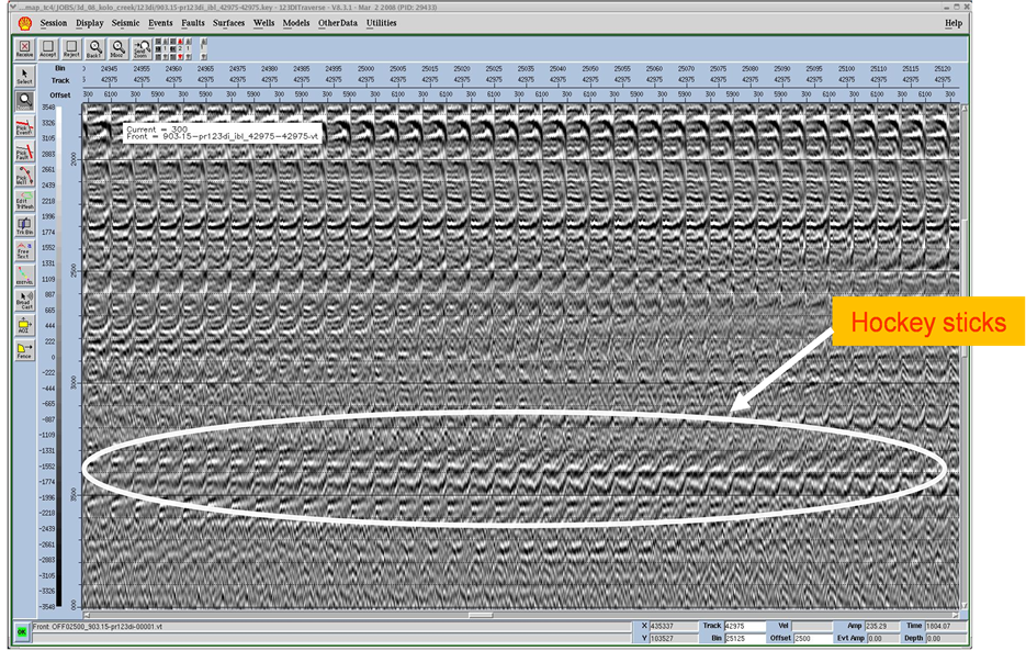
The non-hyperbolic moveout of events in the depobelts is mostly associated with this anisotropy, which is manifested as hockey sticks in seismic records (Figure 2). This phenomenon is usually a common feature of seismic data in Niger delta encountered most especially, when long-offset seismic are employed to illuminate deep targets and get sufficient offset coverage for AVO analysis. This is a consequent of the fact that anisotropy in the depobelts increases with depth.
The aim of the present study therefore, is to estimate ε, δ, γ and η parameters to characterize anisotropy in the depobelts, and finally, derive empirical relations for the estimation of these parameters in the two depobelts.
2. Geology of the Study Area
The stratigraphic sequence of the Niger Delta comprises three broad lithostratigraphic units, namely, a continental shallow massive sand sequence, the Benin Formation, a coastal marine sequence of alternating sands and shales, the Agbada Formation, and a basal marine shale unit, the Akata Formation. Outcrops of these units are exposed at various localities within the Niger delta (Figure 1).
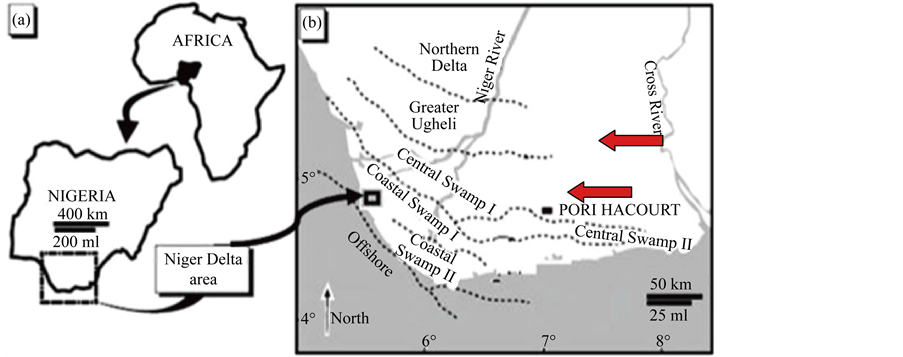
Figure 1. Map of Niger Delta showing the depobelts (study areas are indicated with red arrows).
 (a)
(a)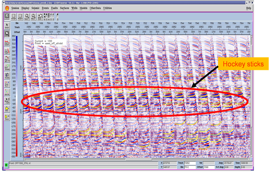 (b)
(b)
Figure 2. Evidence of Anisotropy shown as hockey sticks on seismic gathers acquired in (a) Central Swamp and (b) Greater Ughelli fields of Niger Delta.
The Benin Formation is characterized by high sand percentage (70% - 100%) and forms the top layer of the Niger Delta depositional sequence. The massive sands were deposited in continental environment comprising the fluvial realms (braided and meandering systems) of the upper delta plain. The Agbada Formation consists of alternating sands and shales representing sediments of the transitional environment comprising the lower delta plain (mangrove swamps, floodplain, and marsh) and the coastal barrier and fluviomarine realms. The sand percentage within the Agbada Formation varies from 30% to 70%, which results from the large number of depositional offlap cycles (Obaje, 2005) [4] . The Akata Formation consists of clays and shales with minor sand intercalations. The sediments were deposited in prodelta environments.
Petroleum in the Niger Delta is produced from the unconsolidated sands in the Agbada Formation and the reservoir properties are controlled by depositional environment and agents of deposition, structure and depth of burial.
3. Method of Research
A transversely anisotropic medium with a vertical symmetry are characterized by three anisotropic parameters: ε, γ, and δ (Sayers, 2005 [5] , Jones et. al, 2003 [6] , Kebali and Schmitt, 1995 [7] , Brittan et. al, 1995 [8] ). These are related to the elastic constants by the following equations:
 (1)
(1)
 (2)
(2)
 (3)
(3)
where C11 is the in-plane compressional modulus, C13 is an important constant that controls the shape of the wave surfaces, C33 is the out-of-plane compressional modulus, C44 is the out-of-plane shear modulus and C66 is the in-plane shear modulus. These five independent elastic constants C11, C13, C33, C44 and C66 are for weak and transversely isotropic medium with vertical symmetry.
The P-wave time-processing parameter η (Alkhalifah and Tsvankin, 1995) [3] is expressed as:
 (4)
(4)
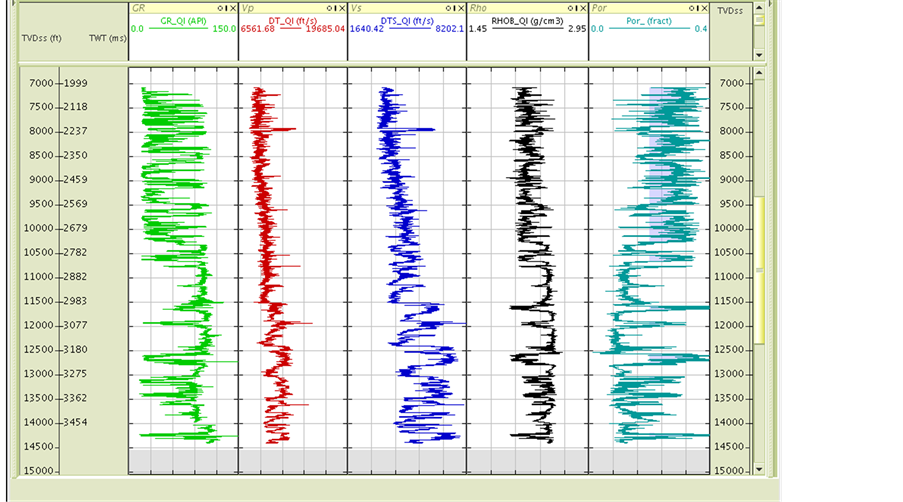
Two wells A and B from each depobelt were used in this study (Figure 3). The wells are comprised of gamma ray (GR), density (RHOB), porosity (POR), dipole sonic compressional (VP) and shear (VS) wave velocity logs. The initial task in the anisotropy modeling is to solve for the five independent elastic constants using well data from which the anisotropy parameters were evaluated using appropriate equations.
4. Presentation of Results
The estimated anisotropy parameters in sands and shales for the two wells were subsequently cross-plotted in shales and sands for the two depobelts to characterize anisotropy.
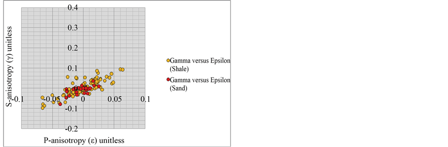
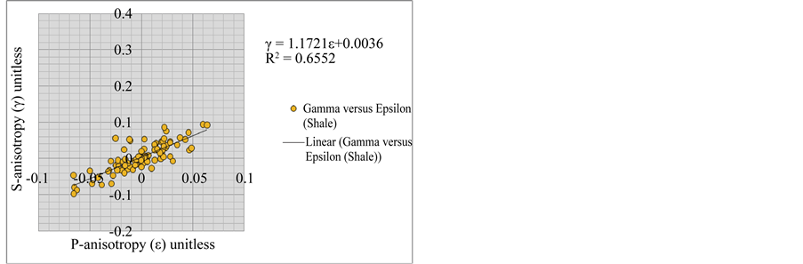
4.1. P-Wave (ε) and S-Wave (γ) Anisotropy Cross-Plots
The P-wave and S-wave anisotropy were cross-plotted for the Central Swamp and Greater Ughelli depobelts (Figure 4 and Figure 5). The γ-ε plot shows that γ is higher than ε in both shale and sand formations caused by the polarization of shear waves in the medium. The plots show significant trend or correlation between P-wave (ε) and S-wave (γ) anisotropies in the two depobelts. The trend is more pronounced in shales being intrinsically anisotropic than sands. Result also show that the best-fit regression line to data for the Central Swamp is
γ = 1.6172ε + 0.0026 with R2 = 0.5177 (5)
and
γ = 1.1721ε + 0.0036 with R2 = 0.6552 (6)
for Greater Ughelli, where ε and γ are the P-wave (ε) and S-wave (γ) anisotropy parameters respectively and R2 is the correlation coefficient.
This empirical relations implies that P-wave (ε) anisotropy can be estimated from S-wave (γ) anisotropy, and vice-versa, once sufficient information about one is known.
4.2. Delta (δ) versus Eta (η) Anisotropy Cross-Plots
Figure 6 and Figure 7 shows the cross-plots of Delta (δ) anisotropy and Eta (η) anisotropy for the Central
 (a)
(a)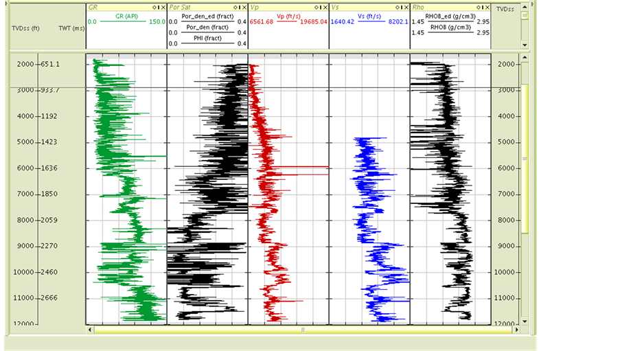 (b)
(b)
Figure 3. Suite of well logs (a) and (b) for the study.
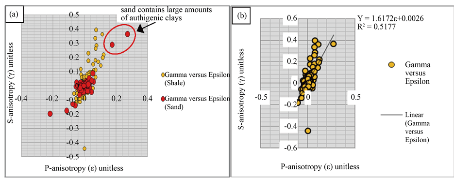
Figure 4. Cross plot of S-anisotropy (γ) versus P-anisotropy (ε) for Well A: (a) for both shale and sand; and (b) for Shale only.
 (a) (b)
Figure 5. Cross plot of S-anisotropy (γ) versus P-anisotropy (ε) for Well B: (a) for shale and sand; and (b) for shale only.
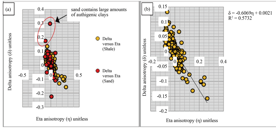
Figure 6. Cross plot of Delta anisotropy (δ) versus Eta anisotropy (η) for Well A: (a) for shale and sand; and (b) for shale only.

Figure 7. Cross plot of Delta anisotropy (δ) versus Eta anisotropy (η) for Well B: (a) for shale and sand; and (b) for sand only
Swamp and Greater Ughelli Depobelts. The result show that η is higher than δ in both sand and shale formations. This behavior could be associated with the alternating sequence of massive shale and sand beds observed within this depobelt. An inverse relationship is observed between the two parameters and the best-fit regression line to data were estimated.
Result show that the best-fit regression line to data for the Central Swamp and Greater Ughelli respectively are:
δ = −0.6069η + 0.0021 with R2 = 0.5732 (7)
and
δ = −0.8586η + 0.0021 with R2 = 0.5165 (8)
5. Discussion of Results
Results from γ-ε cross-plots show that approximately 7% - 29% P-wave anisotropy and 10% - 40% S-wave anisotropy were observed in the shales; while 2.5% - 3% P-wave anisotropy and 2% - 10% S-wave anisotropy were observed in sands. Likewise, in Figure 6 and Figure 7 approximately 10% - 28% Eta ŋ-anisotropy and 8% - 14% Delta δ-anisotropy were observed in the shales; while 8% - 10% Eta ŋ-anisotropy and 5% - 10% Delta δ- anisotropy were observed in sands. This shows that the shales are intrisincally more anisotropic than the sands.
The estimated anisotropy parameters in the Central Swamp is considered to be high (with ε = 29%, γ = 40%, δ = 14%, and ŋ = 28%) as compared to that in Greater Ughelli depobelt (with ε = 7%, γ = 10%, δ = 8%, and δ = 10%).
It is also worthy to note that when a sand contains large amounts of authigenic clays, it may become intrinsically anisotropic (Wang, 2002) [9] . This accounts for the behaviour of sand in Figure 4 and Figure 6 where the sand bodies in Well A (Central Swamp depobelt) shows some traces of anisotropy in γ/ε plots and in δ/ŋ plots respectively. The alternating sequences of sands and shales in the Niger Delta geologically is possibly responsible for this behaviour.
Based on the cross-plots of the anisotropy parameters and analyses of the best-fit regression line of the plots in shale, a relation was derived for ε-γ and δ-η parameters in the two depobelts. These relations are quite good considering their high correlation coefficients. The relations could be used for estimating any of the parameters in the two depobelts once there is appropriate information or data for any one parameter. Such estimation is independent of pressure, pore fluids and lithology.
It is very useful when S-wave (γ) is available, but P-wave (ε) anisotropy is not. This is done to avoid having to undergo the tedious algebraic derivation of the P-wave anisotropy using stiffness tensor. This also applies to δ-η in the study.
6. Conclusions
Our results in the Central Swamp and Greater Ughelli depobelts shows a higher degree of anisotropy in shales than sands, indicating that the Niger Delta shales are intrinsically anisotropic. The predominance of shales in the depobelts accounts for this high degree of anisotropy. The estimated anisotopy is higher in the Central Swamp than the Greater Ughelli depobelt. A relation has also been derived for the P-wave (ε) and S-wave (γ) anisotropies, and also for the Delta δ- and Eta ŋ-anisotropies in the Niger Delta.
The relevance of these parameters in seismic processing and interpretation makes it imperative to have these empirical relations which in effect could be applied in new areas within the Niger Delta to estimate anisotropy parameters for seismic processing and imaging.
Acknowledgements
We are grateful to Shell Petroleum Development Company, Port Harcourt, for the privilege to use their data in this study.
Cite this paper
Iheanyichukwu P. C. Okorie,Joseph O. Ebeniro,Chukwuemeka N. Ehirim, (2016) Anisotropy and Empirical Relations for the Estimation of Anisotropy Parameters in Niger Delta Depobelts. International Journal of Geosciences,07,345-352. doi: 10.4236/ijg.2016.73027
References
- 1. Tsvankin, I., Gaiser, J., Grechka, V., Van der Baan, M. and Thomsen, L. (2010) Seismic Anisotropy in Exploration and Reservoir Characterization: An Overview. Geophysics, 75, 75A15-75A29.
- 2. Thomsen, L. (1986) Weak Elastic Anisotropy. Geophysics, 51, 1954-1966.
http://dx.doi.org/10.1190/1.1442051 - 3. Alkhalifah, T. and Tsvankin, I. (1995) Velocity Analysis for Transversely Isotropic Media. Geophysics, 60, 1550-1566. http://dx.doi.org/10.1190/1.1443888
- 4. Obaje, N.G. (2005) Fairways and Reservoir Prospects of Pliocene—Recent Sands in the Shallows Offshore Niger Delta. Journal of Mining and Geology, 40, 25–38.
- 5. Sayers, C.M. (2005) Seismic Anisotropy of Shales. Geophysical Prospecting, 53, 667-676.
http://dx.doi.org/10.1111/j.1365-2478.2005.00495.x - 6. Jones, I.F., Bridson, M.L. and Bemitsas, N. (2003) Anisotropic Ambiguities in TI Media. First Break, 21, 45-58. http://dx.doi.org/10.3997/1365-2397.2003006
- 7. Kebaili, A. and Schmitt, D.R. (1996)Velocity Anisotry Observed in Wellbore Aeiamicarrivals: Combined Effects of Intrinsic Properties and Layering. Geophysics, 61, 12. http://dx.doi.org/10.1190/1.1443932
- 8. Brittan, J., Wamer, M. and Pratt, G. (1995) Anisotropic Parameters of Layered Media in Terms of Composite Elastic Properties. Geophysics, 60, 1243-1248. http://dx.doi.org/10.1190/1.1443854
- 9. Wang, Z. (2002) Seismic Anisotropy in Sedimentary Rocks, Part 2, Laboratory Data. Geophysics, 67, 1423-1440.
NOTES

*Corresponding author.